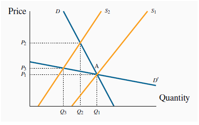
Knowledge of elasticity values is useful in calculating the price change required to eliminate a shortage or surplus. For example, shifts in the supply of agricultural products can create surpluses and shortages. Because of variations in weather conditions, crop yields cannot be forecast accurately. In addition, on account of the low elasticity of demand for such products, low crop yields can increase prices radically, and bumper harvests can have the opposite impact.
Consider Figure
4.4. Econometricians tell us that the demand for foodstuffs is inelastic, so let us operate in the lower (inelastic) part of this demand, D. A change in supply conditions (e.g. a shortage
of rain and a poorer harvest) shifts the supply from  to
to
 with the consequence that the price increases from
  to
to  . In this illustration the price increase is substantial. In contrast, with a relatively flat, or elastic, demand, D', through the
initial point A, the shift in the supply curve has a more moderate impact on the price (from
  to
to  ),
but a relatively larger impact on quantity traded.

In the lower part of the demand curve D, where demand is inelastic, e.g. point A, a shift in supply from  to
to  induces a large percentage increase in price, and a small percentage decrease in quantity demanded. In contrast, for the demand curve D' that goes through the original equilibrium, the region A
is now an elastic region, and the impact of the supply shift is contrary: the %
 P is smaller and the %
 Q is larger.
- 瀏覽次數:2570


