


Consider next the impact of a shift in demand upon the profit maximizing choice of this firm. A rightward shift in demand in Figure 10.6 also yields a new MR curve. The firm therefore chooses a new level of output, using the same profit maximizing rule: set MC = MR. This output will be greater than the previous output, but again the price must be on an elastic portion of the new demand curve. If operating with the same plant size, the MC and ATC curves do not change and the new profit per unit is again read from the ATC curve. The new equilibrium is again defined by where MR = MC.
By this stage the curious student will have asked: “what happens to plant size in the long run?” For example, is the monopolist in Figure 10.6 using the most appropriate plant size in the first place? Even if she is, should the monopolist consider adopting an expanded plant size in response to the shift in demand?
The answer is: in the long run the monopolist is free to choose whatever plant size is best. Her initial plant size might have been optimal for the demand she faced, but if it was, it is unlikely to be optimal for the larger scale of production associated with the demand shift. Accordingly, with the new demand curve, she must consider how much profit she could make using different plant sizes.
To illustrate one possibility, we will think of this firm as having constant returns to scale at all output ranges, as displayed in Figure 10.7. The key characteristic of constant returns to scale is that a doubling of inputs leads to a doubling of output. Therefore, if the per-unit cost of inputs is fixed, a doubling of inputs (and therefore output) leads exactly to a doubling of costs. This implies that, when the firm varies its plant size and its labour use, the cost of producing each additional unit must be constant. The long run marginal cost LMC is therefore constant and equals the ATC
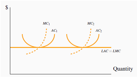
With constant returns to scale and constant prices per unit of labour and capital, a doubling of output involves exactly a doubling of costs. Thus, per unit costs, or average costs, are constant in the LR. Hence LAC = LMC, and each is constant.
Figure 10.8 describes the market
for this good. The optimal output and price are determined in the usual manner: set MC = MR. If the monopolist has plant size corresponding to  , the optimal output is
  and should be sold at the price
  .The key issue now is: given the demand conditions, could the monopolist make more profit by choosing a plant size that differs
from the one corresponding to
.The key issue now is: given the demand conditions, could the monopolist make more profit by choosing a plant size that differs
from the one corresponding to  ?
?
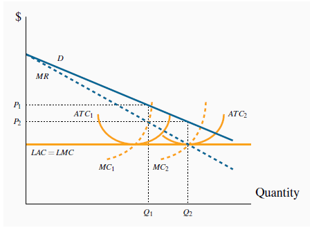
With demand conditions defined by D and MR, the optimal plant size is one corresponding to the point where MR = MC in the long run. Therefore  is the optimal output and the optimal plant size corresponds to
 . If the current plant is defined by
  , then optimal SR production is
  .
.
In this instance the answer is a clear ‘yes’. Her LMC curve is horizontal and so, by increasing output from  to
to  she earns a profit on each additional unit in that range, because the MR curve lies above the LMC curve. In order to produce the output level
  at least cost she must choose a plant size corresponding to
  .
.
- 瀏覽次數:2085
