


Black Diamond Snowboards (BDS) is a start-up snowboard producing enterprise. Its founder has invented a new lamination process that gives extra strength to his boards. He has set up a production line in his garage that has four workstations: laminating, attaching the steel edge, waxing, and packing.
With this process in place, he must examine how productive his firm can be. After extensive testing, he has determined exactly how his productivity depends upon the number of workers. If he employs only one worker, then that worker must perform several tasks, and will encounter ‘down time’ between workstations. Extra workers would therefore not only increase the total output; they could, in addition, increase output per worker. He also realizes that once he has employed a critical number of workers, additional workers may not be so productive: Because they will have to share the fixed amount of machinery in his garage, they may have to wait for another worker to finish using a machine. At such a point, the productivity of his plant will begin to fall off, and he may want to consider capital expansion. But for the moment he is constrained to using this particular assembly plant. Testing leads him to formulate the relationship between workers and output that is described in Table 8.2.
| 1 | 2 | 3 | 4 | 5 |
| Workers | Output (TP) | Marginal product (MPL) | Average product (APL) | Stages of production |
| 0 | 0 | MPL increasing | ||
| 1 | 15 | 15 | 15 | |
| 2 | 40 | 25 | 20 | |
| 3 | 70 | 30 | 23.3 | |
| 4 | 110 | 40 | 27.5 | |
| 5 | 145 | 35 | 29 | MPL positive and declining |
| 6 | 175 | 30 | 29.2 | |
| 7 | 200 | 25 | 28.6 | |
| 8 | 220 | 20 | 27.5 | |
| 9 | 235 | 15 | 26.1 | |
| 10 | 240 | 5 | 24.0 | |
| 11 | 235 | -5 | 21.4 | MPL negative |
By increasing the number of workers in the plant, BDS produces more boards. The relationship between these two variables in columns 1 and 2 in the table is plotted in Figure 8.1. This is called the total product function (TP), and it defines the output produced with different amounts of labour in a plant of fixed size.
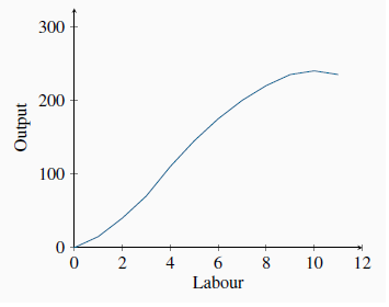
 Total product is the relationship between total
output produced and the number of workers employed, for a given amount of capital.
Total product is the relationship between total
output produced and the number of workers employed, for a given amount of capital.
This relationship is positive, indicating that more workers produce more boards. But the curve has an interesting pattern. In the initial expansion of employment it becomes progressively steeper – its curvature is slightly convex; following this phase the function’s increase becomes progressively less steep – its curvature is concave. These different stages in the TP curve tell us a great deal about productivity in BDS. To see this, consider the additional number of boards produced by each worker. The first worker produces 15. When a second worker is hired, the total product rises to 40, so the additional product attributable to the second worker is 25. A third worker increases output by 30 units, and so on. We refer to this additional output as the marginal product (MP) of an additional worker, because it defines the incremental, or marginal, contribution of the worker. These values are entered in column 3.
More generally the MP of labour is defined as the change in output divided by the change in the number of units of labour employed. Using the Greek capital delta (D) to denote a change, we can
define

In this example the change in labour is one unit at each stage and hence the marginal product of labour is simply the corresponding change in output. It is also the case that the  is the slope of the TP curve – the change in the value on the vertical axis
due to a change in the value of the variable on the horizontal axis.
is the slope of the TP curve – the change in the value on the vertical axis
due to a change in the value of the variable on the horizontal axis.
Marginal product of labour is the addition
to output produced by each additional worker. It is also the slope of the total product curve.
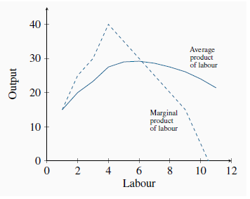
During the initial stage of production expansion, the marginal product of each worker is increasing. It increases from 15 to 40 as BDS moves from having one employee to four employees. We can think of this increasing MP as being made possible by the fact that each worker is able to spend more time at his workstation, and less time moving between tasks. But, at a certain point in the employment expansion, the MP reaches a maximum and then begins to tail off. At this stage – in the concave region of the TP curve – additional workers continue to produce additional output, but at a diminishing rate. For example, while the fourth worker adds 40 units to output, the fifth worker adds 35, the sixth worker 30, and so on. This declining MP is due to the constraint of a fixed number of machines: All workers must share the same capital. The MP function is plotted in Figure 8.2.
The phenomenon we have just described has the status of a law in economics: The law of diminishing returns states that, in the face of a fixed amount of capital, the contribution of additional units of a variable factor must eventually decline.
Law of diminishing returns: when increments of a
variable factor (labour) are added to a fixed amount of another factor (capital), the marginal product of the variable factor must eventually decline.
The relationship between Figure 8.1 and Figure 8.2 should be noted. First, the reaches a maximum at an output of 4 units – where the slope of the TP curve is greatest. The MPL curve remains positive beyond this output, but declines: The TP curve reaches a maximum when the tenth unit of labour is employed. An eleventh unit actually reduces total output; therefore, the MP of this eleventh worker is negative! In Figure 8.2, the MP curve becomes negative at this point. The garage is now so crowded with workers that they are beginning to obstruct the operation of the production process. Thus the producer would never employ an eleventh unit of labour.
Next, consider the information in the fourth column of the table. It defines the average product of labour (APL)—the amount of output produced, on average, by workers at different employment levels:

This function is also plotted in Figure 8.2. Referring to the table: the AP column indicates, for example, that when two units of labour are employed and forty units of output are produced, the average production level of each worker is 20 units (=40/2). When three workers produce 70 units, their average production is 23.3 (=70/3), and so forth. Like theMP function, this one also increases and subsequently decreases, reflecting exactly the same productivity forces that are at work on the MP curve.
Average product of labour is the number of units
of output produced per unit of labour at different levels of employment.
The AP and MP functions intersect at the point where the AP is at its peak. This is no accident, and has a simple explanation. Imagine a baseball player who is batting .280 coming into today’s game—he has been hitting his way onto base 28 percent of the time when he goes up to bat, so far this season. This is his average product, AP.
| Workers | Output | Capital Cost Fixed | Labour Cost Variable | Total Costs | Average Fixed Cost | Average Variable Cost | Average Total Cost | Marginal Cost |
| 0 | 0 | 3,000 | 0 | 3,000 | ||||
| 1 | 15 | 3,000 | 1,000 | 4,000 | 200.0 | 666.7 | 266.7 | 66.7 |
| 2 | 40 | 3,000 | 2,000 | 5,000 | 75.0 | 50.0 | 125.0 | 40.0 |
| 3 | 70 | 3,000 | 3,000 | 6,000 | 42.9 | 42.9 | 85.7 | 33.3 |
| 4 | 110 | 3,000 | 4,000 | 7,000 | 27.3 | 36.4 | 63.6 | 25.0 |
| 5 | 145 | 3,000 | 5,000 | 8,000 | 20.7 | 34.5 | 55.2 | 28.6 |
| 6 | 175 | 3,000 | 6,000 | 9,000 | 17.1 | 34.3 | 51.4 | 33.3 |
| 7 | 200 | 3,000 | 7,000 | 10,000 | 15.0 | 35.0 | 50.0 | 40.0 |
| 8 | 220 | 3,000 | 8,000 | 11,000 | 13.6 | 36.4 | 50.0 | 50.0 |
| 9 | 235 | 3,000 | 9,000 | 12,000 | 12.8 | 38.3 | 51.1 | 66.7 |
| 10 | 240 | 3,000 | 10,000 | 13,000 | 12.5 | 41.7 | 54.2 | 28.6 |
In today’s game, if he bats .500 (he hits his way to base on half of his at-bats), then he will improve his average. Today’s batting (his MP) at .500 therefore pulls up his season’s AP. Accordingly, whenever the MP exceeds the AP, the AP is pulled up. By the same reasoning, if his MP is less than his season average, his average will be pulled down. It follows that the two functions must intersect at the peak of the AP curve. Noting that the inequality sign always points to the smaller value, we can make the following summary statement:
If MP > AP, then AP increases; if MP < AP, then AP declines.
While the owner of BDS may understand his productivity relations, his ultimate goal is to make profit, and for this he must figure out how productivity translates into cost.
- 2696 reads
