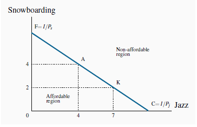
Neal’s monthly expenditure limit, or budget constraint, is $200. In addition, he faces a price of $30 for lift tickets and $20 per visit to jazz clubs. Therefore, using S to denote the number of snowboard outings and J the number of jazz club visits, if he spends his entire budget it must be true that the sum of expenditures on each activity exhausts his budget or income (I):
$30S+$20J = $200
or, more generally, that the budget constraint is defined by

(6.3)
whatever the income and prices may be. Since many different combinations of the two goods are affordable, it follows that the budget constraint defines all bundles of goods that the consumer can afford with a given budget.
 The budget constraint defines all bundles of
goods that the consumer can afford with a given budget.
The budget constraint, then, is just what it claims to be—a limit on behaviour. Neal’s budget constraint is illustrated in Figure 6.6, where the amount of each good consumed is given on the axes. If he spends all of his $200 income on jazz, he can make exactly ten jazz club visits ($200/$20= 10). The calculation also applies to visits to Whistler. The intercept value is always obtained by dividing income by the price of the good or activity in question.

FC is the budget constraint and defines the affordable combinations of snowboarding and jazz. F represents all income spent on snowboarding. Thus F= I=Ps. Similarly C= I= . Points above FC are not attainable. The slope
  . The affordable set is
0FC.
In addition to these affordable extremes, Neal can also afford many other bundles, e.g., (S = 2, J =7), or (S = 4, J = 4), or (S = 6, J = 1). The set of feasible, or affordable, combinations is bounded by the budget line, and this is illustrated in Figure 6.6.
 The affordable set of goods and services for
the consumer is bounded by the budget line from above; the non-affordable set lies strictly above the budget line.
The slope of the budget line is informative. It indicates how many snowboard visits must be sacrificed for one additional jazz visit; it defines the consumer’s trade-offs. To illustrate: Suppose Neal is initially at point A (J = 4,S = 4), and moves to point K (J = 7,S = 2). Clearly, both points are affordable. In making the move, he trades two snowboard outings in order to get three additional jazz club visits, a trade-off of 2/3. This trade-off is the slope of the budget line, which, in Figure 6.6, is AB/BK = -2/3, where the negative sign reflects the downward slope.
Could it be that this ratio reflects the two prices ($20/$30)? The answer is yes: If each unit of the good on the vertical axis is more expensive than the good on the horizontal axis, it makes
sense that fewer units of the former must be sacrificed to get one unit of the latter. This result is derived by noting that the slope of the budget line is given by the vertical distance
divided by the horizontal distance, OF/OC. The points F and C were obtained by dividing income by the respective price— remember that the jazz intercept is $200/$20 = 10. Formally, that is
I= . The intercept on the snowboard axis is likewise I=
 . We can write the condition that the slope of the budget constraint be equal to the
vertical distance divided by the horizontal distance as

Since the budget line has a negative slope, it is technically correct to define it with a negative sign. But, as with elasticities, the sign is frequently omitted. In the general case for two goods where good x is on the horizontal axis, and y on the vertical axis, the slope is therefore defined as:
Slope of the budget constraint 
(6.4)
Note that the properties of the budget constraint can also be obtained by rewriting Equation 6.3. Bringing the term PjJ to the right-hand side yields

Dividing through by Ps results in

(6.5)
From Theories, models and data we know that if S is on
the vertical axis then (I= ) is the vertical axis intercept, and the
negative of price ratio (
 /
/  ) is the slope of the constraint.
- 瀏覽次數:2704


