Monopolistic competition presumes a large number of quite small producers or suppliers, each of whom may have a slightly differentiated product. The competition element of this name signifies that there are many participants, while the monopoly component signifies that each supplier faces a downward sloping demand. In concrete terms, your local coffee shop that serves “fair trade” coffee has a product that differs slightly from that of neighbouring shops that sell the traditional product. They coexist in the same sector, and probably charge different prices: The fair trade supplier likely charges a higher price, but knows nonetheless that too large a difference between her price and the prices of her competitors will see some of her clientele migrate to those lowerpriced establishments. That is to say, she faces a downward-sloping demand curve.
The competition part of the name also indicates that there is free entry and exit. There are no barriers to entry. As a consequence, we know at the outset that only normal profits will exist in a long-run equilibrium. Economic profits will be competed away by entry, just as losses will erode due to exit.
As a general rule then, each firm can influence its market share to some extent by changing its price. Its demand curve is not horizontal because different firms’ products are only limited substitutes. A lower price level may draw some new customers away from competitors, but convenience or taste will prevent most patrons from deserting their local businesses. In concrete terms: a pasta special at the local Italian restaurant that reduces the price below the corresponding price at the competing local Thai restaurant will indeed draw clients away from the latter, but the foods are sufficiently different that not all customers will leave the Thai restaurant. The differentiated menus mean that many customers will continue to pay the higher price.
 A differentiated product is one that differs
slightly from other products in the same market.
Given that there are very many firms, the theory also envisages limits to scale economies. Firms are small and, with many competitors, individual firms do not compete strategically with particular rivals. Because the various products offered are slightly differentiated, we avoid graphics with a market demand, because this would imply that a uniform product is being considered. At the same time the market is a well-defined concept—it might be composed of all those restaurants within a reasonable distance, for example, even though each restaurant is slightly different from the others.
The market share of each firm depends on the price that it charges and on the number of competing firms. For a given number of suppliers, a shift in industry demand also shifts the demand facing each firm. Likewise, the presence of more firms in the industry reduces the demand facing each one.
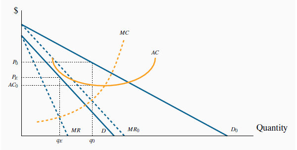
The market equilibrium is illustrated in Figure 11.2. Here Do is the initial demand facing a representative firm, and MR0 is the corresponding marginal revenue curve. Profit is maximized where MC = MR, and the price Po is obtained from the demand curve corresponding to the output q0. Total profit is the product of output times the difference between price and average cost, which equals qoX(Po - ACo).

Profits exist at the initial equilibrium (qo,Po). Hence, new firms enter and reduce the share of the total market faced by each firm, thereby shifting back their demand curve. A final
equilibrium is reached where economic profits are eliminated: at AC =  and MR = MC.
With free entry, such profits attract new firms. The increased number of firms reduces the share of the market that any one firm can claim. That is, the firm’s demand curve shifts inwards when
entry occurs. As long as (economic) profits exist, this process continues. For entry to cease, average costs must equal price. A final equilibrium is illustrated by the combination ( ,
, ), where the demand has shifted inward to D.
At this long-run equilibrium, two conditions must hold: First, the optimal pricing rule must be satisfied—that is MC = MR; second it must be the case that only normal profits are made at the final equilibrium. Economic profits are competed away as a result of free entry. And these two conditions must exist at the optimal output. Graphically this implies that ATC must equal price at the output where MC = MR. In turn this implies that the ATC is tangent to the demand curve where P = ATC. While this could be proven mathematically, it is easy to intuit why this tangency must exist: If ATC merely intersected the demand curve at the output where MC = MR, we could find some other output where the demand price would be above ATC, suggesting that profits could be made at such an output. Clearly that could not represent an equilibrium.
 The monopolistically competitive equilibrium in
the long run requires the firm’s demand curve to be tangent to the ATC curve at the output where MR = MC.
- 瀏覽次數:4135


