


Neal loves to pump his way through the high-altitude powder at the Whistler ski and snowboard resort. His student-rate lift-ticket cost is $30 per visit. He also loves to frequent the jazz bars in downtown Vancouver, and each such visit costs him $20. With expensive passions, Neal must allocate his monthly entertainment budget carefully. He has evaluated how much satisfaction, measured in utils, he obtains from each snowboard outing and each jazz club visit. We assume that these utils are measurable, and use the term cardinal utility to denote this. These measurable utility values are listed in columns 2 and 3 of Table 6.1. They define the total utility he gets from various amounts of the two activities.
| 1 | 2 | 3 | 4 | 5 | 6 | 7 |
| Visit # | Total snowboard utils | Total jazz utils | Marginal snowboard utils | Marginal jazz utils | Marginal snowboard utils per $ | Marginal jazz utils per $ |
| 1 | 72 | 52 | 72 | 52 | 2.4 | 2.6 |
| 2 | 132 | 94 | 60 | 42 | 2.0 | 2.1 |
| 3 | 182 | 128 | 50 | 34 | 1.67 | 1.7 |
| 4 | 224 | 156 | 42 | 28 | 1.4 | 1.4 |
| 5 | 260 | 180 | 36 | 24 | 1.2 | 1.2 |
| 6 | 292 | 201 | 32 | 21 | 1.07 | 1.05 |
| 7 | 321 | 220 | 19 | 19 | 0.97 | 0.95 |
Price of snowboard visit=$30. Price of jazz club visit=$20.
 Cardinal utility is a measurable concept of
satisfaction.
Cardinal utility is a measurable concept of
satisfaction.
Total utility is a measure of the total
satisfaction derived from consuming a given amount of goods and services.
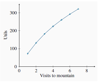
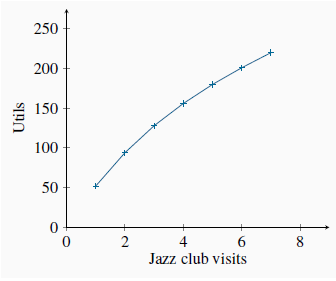
Neal’s total utility from each activity in this example is independent of the amount of the other activity he engages in. These total utilities are also plotted in Figure 6.1 and Figure 6.2. Clearly, more of each activity yields more utility, so the additional or marginal utility (MU) of each activity is positive. This positive marginal utility for any amount of the good consumed, no matter how much, reflects the assumption of non-satiation—more is always better. Note, however, that the decreasing slopes of the total utility curves show that total utility is increasing at a diminishing rate. While more is certainly better, each additional visit to Whistler or a jazz club augments Neal’s utility by a smaller amount. At the margin, his additional utility declines: he has diminishing marginal utility. The marginal utilities associated with snowboarding and jazz are entered in columns 4 and 5 of Table 6.1. They are the differences in total utility values when consumption increases by one unit. For example, when Neal makes a sixth visit to Whistler his total utility increases from 260 utils to 292 utils. His marginal utility for the sixth unit is therefore 32 utils, as defined in column 4. In light of this example, it should be clear that we can define marginal utility as:

(6.1)
where Dx denotes the change in the quantity consumed of the good or service in question.
Marginal utility is the addition to total utility
created when one more unit of a good or service is consumed.
Diminishing marginal utility implies that the
addition to total utility from each extra unit of a good or service consumed is declining.
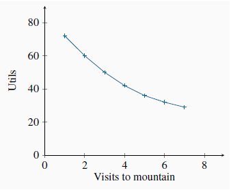
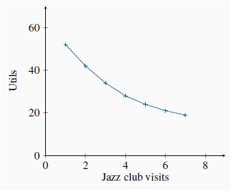
The marginal utilities associated with consuming different amounts of the two goods are plotted in Figure 6.3 and Figure 6.4, using the data from columns 4 and 5 in Table 6.1. These functions are declining, as indicated by their negative slope. It should also be clear that the MU curves can be derived from the TU curves because, from Equation 6.1, the MU is the slope of the TU curve. For example, when visits to the mountain increase from three to four, TU increases from 182 to 224. Hence MU = (224 - 182)/1 = 42, which is the value of the fourth visit plotted in Figure 6.3.
Now that Neal has defined his utility schedules, he must consider the price of each activity. Ultimately, when deciding how to allocate his monthly entertainment budget, he must evaluate how much utility he gets from each dollar spent on snowboarding and jazz: What “bang for his buck” does he get? Let us see how he might go about allocating his budget. When he has fully spent his budget in the manner that will yield him greatest utility, we say that he has attained equilibrium, because he will have no incentive to change his expenditure patterns.
If he boards once, at a cost of $30, he gets 72 utils of satisfaction, which is 2.4 utils per dollar spent (= 72/30). One visit to a jazz club would yield him 2.6 utils per dollar (= 52/20). Initially, therefore, his dollars give him more utility per dollar when spent on jazz. His MU per dollar spent on each activity is given in the final two columns of the table. These values are obtained by dividing the MU associated with each additional unit by the good’s price.
We will assume that Neal has a budget of $200. He realizes that his initial expenditure should be on a jazz club visit, because he gets more utility per dollar spent there. Having made one such expenditure, he sees that a second outing would yield him 2.1 utils per dollar expended, while a first visit to Whistler would yield him 2.4 utils per dollar. Accordingly, his second activity is a snowboard outing.
Having made one jazz and one snowboarding visit, he then decides upon a second jazz club visit for the same reason as before—utility value for his money. He continues to allocate his budget in this way until his budget is exhausted. In our example, this occurs when he spends $120 on four snowboarding outings and $80 on four jazz club visits. At this consumer equilibrium, he gets the same utility value per dollar for the last unit of each activity consumed. This is a necessary condition for him to be maximizing his utility, that is, to be in equilibrium.
Consumer equilibrium occurs when marginal utility
per dollar spent on the last unit of each good is equal.
To be absolutely convinced of this, imagine that Neal had chosen instead to board twice and to visit the jazz clubs seven times; this combination would also exhaust his $200 budget exactly. With such an allocation, he would get 2.0 utils per dollar spent on his marginal (second) snowboard outing, but just 0.95 utils per dollar spent on his marginal (seventh) jazz club visit. 1 If, instead, he were to reallocate his budget in favour of snowboarding, he would get 1.67 utils per dollar spent on a third visit to the hills. By reducing the number of jazz visits by one, he would lose 0.95 utils per dollar reallocated. Consequently, the utility gain from a reallocation of his budget towards snowboarding would outweigh the utility loss from allocating fewer dollars to jazz. His initial allocation, therefore, was not an optimum, or equilibrium.
Only when the utility per dollar expended on each activity is equal at the margin will Neal be optimizing. When that condition holds, a reallocation would be of no benefit to him, because the gains from one more dollar on boarding would be exactly offset by the loss from one dollar less spent on jazz. Therefore, we can write the equilibrium condition as
(6.2)
While this example has just two goods, in the more general case of many goods, this same condition must hold for all pairs of goods on which the consumer allocates his or her budget.
- 3342 reads
