


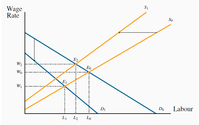
The fact that labour is a derived demand is what distinguishes the labour market’s dynamics from the goods-market dynamics. Let us investigate these dynamics with the help of Figure 12.4; it contains supply and demand functions for one particular industry – the cement industry let us assume.
A fall in the price of the good produced in a particular industry reduces the value of the  . Demand for labour thus falls from
  to
to  and a new equilibrium
  results. Alternatively, from
  , an increase in wages in another sector of the economy induces some labour to move to that sector. This is represented by the
shift of S0 to S1 and the new equilibrium
, an increase in wages in another sector of the economy induces some labour to move to that sector. This is represented by the
shift of S0 to S1 and the new equilibrium  .
.
In Figure 12.1 we illustrated
the impact on the demand for labour of a decline in the price of the output produced. In the current example, suppose that the demand for cement declines as a result of a slowdown in the
construction sector, which in turn results in a fall in the cement price. The impact of this price fall is to reduce the output value of each worker in the cement producing industry, because
their output now yields a lower price. This decline in the VMPL is represented in Figure 12.4 as a shift from  to
to  . The new VMPL curve (
 ) results in the new equilibrium
  .
.
As a second example: suppose the demand for labour in some other sectors of the economy increases and its wage in those sectors rises correspondingly, this is reflected in the cement sector as
a backward shift in the supply of labour (some other price has changed and results in a shift in the labour supply curve). In Figure 12.4 supply shifts from  to
to  and the equilibrium goes from
  to
to .
.
How large are these impacts likely to be? That will depend upon how mobile labour is between sectors: spillover effects will be smaller if labour is less mobile. This brings us naturally to the concepts of transfer earnings and rent.
Consider the case of a performing violinist whose wage is $80,000. If, as a best alternative, she can earn $60,000 as a music teacher then her rent is $20,000 and her transfer earnings $60,000: her rent is the excess she currently earns above the best alternative. Another violinist in the same orchestra, earning the same amount, who could earn $65,000 as a teacher has rent of $15,000. The alternative is called the reservation wage. The violinists should not work in the orchestra unless they earn at least what they can earn in the next best alternative.
 Transfer earnings are the amount that an
individual can earn in the next highest paying alternative job.
Transfer earnings are the amount that an
individual can earn in the next highest paying alternative job.
 Rent is the excess remuneration an individual
currently receives above the next best alternative. This alternative is the reservation wage.
Rent is the excess remuneration an individual
currently receives above the next best alternative. This alternative is the reservation wage.
These concepts are illustrated in Figure 12.5 for a large number of individuals. In this illustration, different individuals are willing to work for different amounts, but all are paid the same wage
Wo. The market labour supply curve by definition defines the wage for which each individual is willing to work. Thus the rent earned by labour in this market is the sum of the excess of the
wage over each individual’s transfer earnings – the area  . This
area is also what we called producer or supplier surplus in Welfare economics and externalities.
. This
area is also what we called producer or supplier surplus in Welfare economics and externalities.
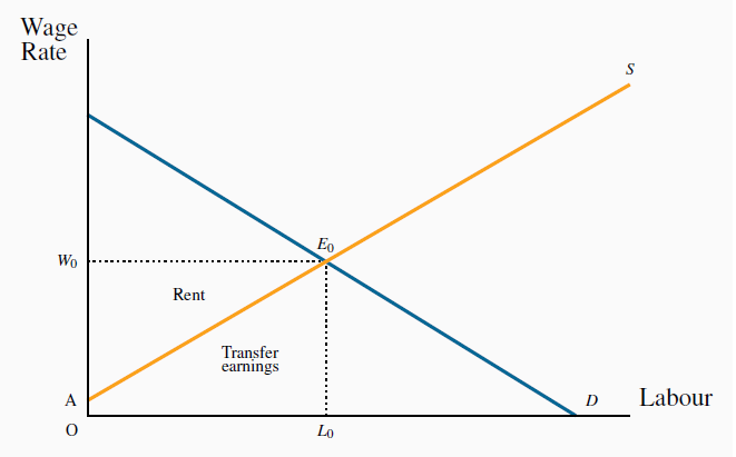
Rent is the excess of earnings over reservation wages. Each individual earns  and is willing to work for the amount defined by the labour supply curve. Hence rent is
  and transfer earnings
  . Rent is thus the term for supplier surplus in this market.
- 3225 reads
