


Figure 12.8 illustrates
the market for capital services for a particular industry. The long-run equilibrium is at Eo where the supply intersects the industry demand Do. Demand is derived from the firms’  schedules, and we have assumed that the supply to this particular industry
is infinitely elastic. Ko units of capital services are traded at the rental rate Ro. This rate must correspond to the rate of return obtained in the economy at large in equilibrium: if returns
in this sector were lower than the returns available elsewhere we would expect capital to migrate to those sectors where the return is higher; conversely if returns were higher.
schedules, and we have assumed that the supply to this particular industry
is infinitely elastic. Ko units of capital services are traded at the rental rate Ro. This rate must correspond to the rate of return obtained in the economy at large in equilibrium: if returns
in this sector were lower than the returns available elsewhere we would expect capital to migrate to those sectors where the return is higher; conversely if returns were higher.
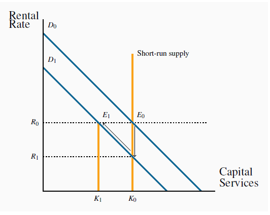
From the equilibrium Eo, a drop in the demand for capital services in a specific industry from Do to D drives the return on its capital Ko down to R
 . This is lower than the economy wide return Ro. No new investment takes place in the sector; capital depreciates and the stock
ultimately falls to K
. This is lower than the economy wide return Ro. No new investment takes place in the sector; capital depreciates and the stock
ultimately falls to K , where the return again equals Ro.
Suppose now there is a slowdown in this industry that reduces the demand for capital services from Do to D , yielding a new equilibrium E
 . However, this new equilibrium cannot be attained immediately: while firms may be able to unload some of their capital, such as
trucks, much of their capital is fixed in place. Firms cannot readily offload buildings or machinery designed for a specific purpose. Instead capital depreciates over time from Ko to K
. However, this new equilibrium cannot be attained immediately: while firms may be able to unload some of their capital, such as
trucks, much of their capital is fixed in place. Firms cannot readily offload buildings or machinery designed for a specific purpose. Instead capital depreciates over time from Ko to K and gradually attains the new equilibrium E
 , where once again the sector is earning the return available in the economy at large, Ro.
- 2219 reads
