


We could now examine all four components of planned spending separately. [***Different chapters of this book delve deeper into these types of spending.***] For the moment, however, we group them all together. We focus on the fact that total planned spending depends positively on the level of income and output in an economy, for two main reasons:
- If households have higher income, they are likely to increase their spending on many goods and services. The relationship between income and consumption is one of the cornerstones of macroeconomics.
- Firms are likely to decide that higher levels of output—particularly if expected to persist— mean that they should build up their capital stock and thus increase their investment.
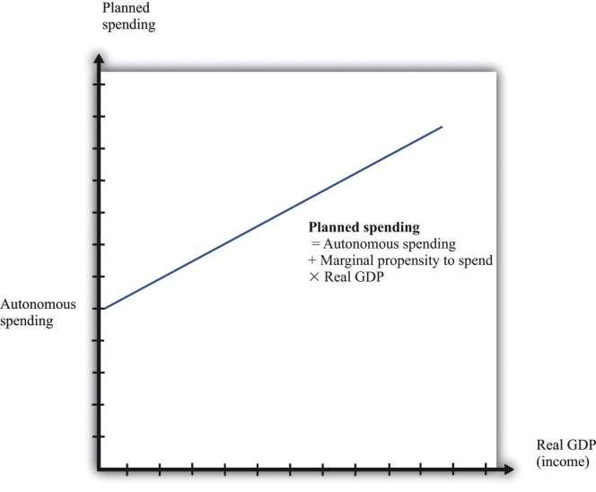
In summary, we conclude that when income increases, planned expenditure also increases. We illustrate this in ****Figure 7.8 "The Planned Spending Line", where we suppose for simplicity that the relationship between planned spending and GDP is a straight line: planned spending = autonomous spending + marginal propensity to spend × GDP.
Autonomous spending is the intercept of the planned spending line. It is the amount of spending that there would be in an economy if income were zero. It is positive, for two reasons: (1) A household with no income still wants to consume something, so it will either draw on its existing savings or borrow against future income. (2) The government purchases goods and services even if income is zero.
The marginal propensity to spend is the slope of the planned spending line. It tells us how much planned spending increases if there is a $1 increase in income. The marginal propensity to spend is positive: Increases in income lead to increased spending by households and firms. The marginal propensity to spend is less than one, largely because of consumption smoothing by households. If household income increases by $1, households typically consume only a fraction of the increase, saving the remainder to finance future consumption. This equation, together with the condition that GDP equals planned spending, gives us the aggregate expenditure model.
Toolkit: Section 16.19 "The Aggregate Expenditure Model"
The aggregate expenditure model takes as its starting point the fact that GDP measures both total spending and total production. The model focuses on the relationships between output and spending, which we write as follows:
planned spending = GDP
and
planned spending = autonomous spending + marginal propensity to spend × GDP.
The model finds the value of output for a given value of the price level. It is then combined with a model of price adjustment to give a complete picture of the economy.
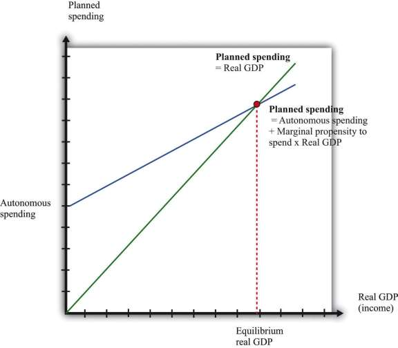
Figure 7.9 Equilibrium in the Aggregate Expenditure Model
The aggregate expenditure framework tells us that the economy is in equilibrium when planned spending equals real GDP.
We can solve the two equations to find the values of GDP and planned spending that are consistent with both equations:
We can also take a graphical approach, as shown in ***Figure 7.9 "Equilibrium in the Aggregate Expenditure Model". On the horizontal axis is the level of real GDP, while on the vertical axis is the overall level of (planned) spending in the economy. We graph the two relationships of the aggregate expenditure model. The first line is a 45° line—that is, it is a line with a slope equal to one and passing through the origin. The second is the planned spending line. The point that solves the two equations is the point where the two lines intersect. This diagram is the essence of the aggregate expenditure model of the macroeconomy.
The aggregate expenditure model makes no reference to potential output or the supply side of the economy. The model assumes that the total amount of output produced will always equal the quantity demanded at the given price. You might think that this neglect of the supply side is a weakness of the model, and you would be right. In Section 7.4.6 "Price Adjustment", when we introduce the adjustment of prices, the significance of potential output becomes clear.
- 9110 reads
