


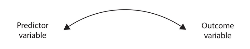
In contrast to descriptive research, which is designed primarily to provide static pictures, correlational research involves the measurement of two or more relevant variables and an assessment of the relationship between or among those variables. For instance, the variables of height and weight are systematically related (correlated) because taller people generally weigh more than shorter people. In the same way, study time and memory errors are also related, because the more time a person is given to study a list of words, the fewer errors he or she will make. When there are two variables in the research design, one of them is called the predictor variable and the other the outcome variable. The research design can be visualized like this, where the curved arrow represents the expected correlation between the two variables:
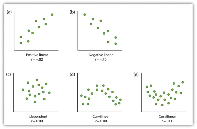
One way of organizing the data from a correlational study with two variables is to graph the values of each of the measured variables using a scatter plot. As you can see in Figure 2.8, a scatter plot is a visual image of the relationship between two variables. A point is plotted for each individual at the intersection of his or her scores for the two variables. When the association between the variables on the scatter plot can be easily approximated with a straight line, as in parts (a) and (b) of Figure 2.8, the variables are said to have a linear relationship.
When the straight line indicates that individuals who have above-average values for one variable also tend to have above-average values for the other variable, as in part (a), the relationship is said to be positive linear. Examples of positive linear relationships include those between height and weight, between education and income, and between age and mathematical abilities in children. In each case people who score higher on one of the variables also tend to score higher on the other variable. Negative linear relationships, in contrast, as shown in part (b), occur when above-average values for one variable tend to be associated with below-average values for the other variable. Examples of negative linear relationships include those between the age of a child and the number of diapers the child uses, and between practice on and errors made on a learning task. In these cases people who score higher on one of the variables tend to score lower on the other variable.
Relationships between variables that cannot be described with a straight line are known as nonlinear relationships. Part (c) of Figure 2.8 shows a common pattern in which the distribution of the points is essentially random. In this case there is no relationship at all between the two variables, and they are said to be independent. Parts (d) and (e) of Figure 2.8 show patterns of association in which, although there is an association, the points are not well described by a single straight line. For instance, part (d) shows the type of relationship that frequently occurs between anxiety and performance. Increases in anxiety from low to moderate levels are associated with performance increases, whereas increases in anxiety from moderate to high levels are associated with decreases in performance. Relationships that change in direction and thus are not described by a single straight line are called curvilinear relationships.
Source: Adapted from Stangor, C. (2011). Research methods for the behavioral sciences (4th ed.). Mountain View, CA: Cengage.
The most common statistical measure of the strength of linear relationships among variables is the Pearson correlation coefficient, which is symbolized by the letter r. The value of the correlation coefficient ranges from r= –1.00 to r = +1.00. The direction of the linear relationship is indicated by the sign of the correlation coefficient. Positive values of r (such as r = .54 or r = .67) indicate that the relationship is positive linear (i.e., the pattern of the dots on the scatter plot runs from the lower left to the upper right), whereas negative values of r (such as r = –.30 or r = –.72) indicate negative linear relationships (i.e., the dots run from the upper left to the lower right). The strength of the linear relationship is indexed by the distance of the correlation coefficient from zero (its absolute value). For instance, r = –.54 is a stronger relationship than r= .30, and r = .72 is a stronger relationship than r = –.57. Because the Pearson correlation coefficient only measures linear relationships, variables that have curvilinear relationships are not well described by r, and the observed correlation will be close to zero.
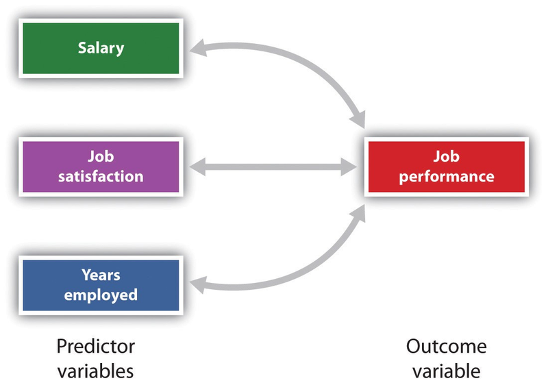
It is also possible to study relationships among more than two measures at the same time. A research design in which more than one predictor variable is used to predict a single outcome variable is analyzed through multiple regression (Aiken & West, 1991). 1 Multiple regression is a statistical technique, based on correlation coefficients among variables, that allows predicting a single outcome variable from more than one predictor variable. For instance, Figure 2.9 shows a multiple regression analysis in which three predictor variables are used to predict a single outcome. The use of multiple regression analysis shows an important advantage of correlational research designs—they can be used to make predictions about a person’s likely score on an outcome variable (e.g., job performance) based on knowledge of other variables.
An important limitation of correlational research designs is that they cannot be used to draw conclusions about the causal relationships among the measured variables. Consider, for instance, a researcher who has hypothesized that viewing violent behavior will cause increased aggressive play in children. He has collected, from a sample of fourth-grade children, a measure of how many violent television shows each child views during the week, as well as a measure of how aggressively each child plays on the school playground. From his collected data, the researcher discovers a positive correlation between the two measured variables.
Although this positive correlation appears to support the researcher’s hypothesis, it cannot be taken to indicate that viewing violent television causes aggressive behavior. Although the researcher is tempted to assume that viewing violent television causes aggressive play,

there are other possibilities. One alternate possibility is that the causal direction is exactly opposite from what has been hypothesized. Perhaps children who have behaved aggressively at school develop residual excitement that leads them to want to watch violent television shows at home:

Although this possibility may seem less likely, there is no way to rule out the possibility of such reverse causation on the basis of this observed correlation. It is also possible that both causal directions are operating and that the two variables cause each other:

Still another possible explanation for the observed correlation is that it has been produced by the presence of a common-causal variable (also known as a third variable). A common-causal variable is a variable that is not part of the research hypothesis but that causes both the predictor and the outcome variable and thus produces the observed correlation between them. In our example a potential common-causal variable is the discipline style of the children’s parents. Parents who use a harsh and punitive discipline style may produce children who both like to watch violent television and who behave aggressively in comparison to children whose parents use less harsh discipline:
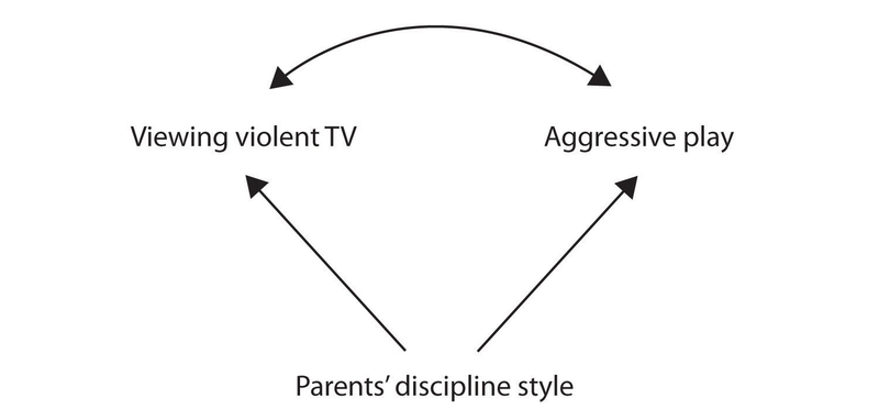
In this case, television viewing and aggressive play would be positively correlated (as indicated by the curved arrow between them), even though neither one caused the other but they were both caused by the discipline style of the parents (the straight arrows). When the predictor and outcome variables are both caused by a common-causal variable, the observed relationship between them is said to be spurious. A spurious relationship is a relationship between two variables in which a common-causal variable produces and “explains away” the relationship. If effects of the common-causal variable were taken away, or controlled for, the relationship between the predictor and outcome variables would disappear. In the example the relationship between aggression and television viewing might be spurious because by controlling for the effect of the parents’ disciplining style, the relationship between television viewing and aggressive behavior might go away.
Common-causal variables in correlational research designs can be thought of as “mystery” variables because, as they have not been measured, their presence and identity are usually unknown to the researcher. Since it is not possible to measure every variable that could cause both the predictor and outcome variables, the existence of an unknown common-causal variable is always a possibility. For this reason, we are left with the basic limitation of correlational research: Correlation does not demonstrate causation. It is important that when you read about correlational research projects, you keep in mind the possibility of spurious relationships, and be sure to interpret the findings appropriately. Although correlational research is sometimes reported as demonstrating causality without any mention being made of the possibility of reverse causation or common-causal variables, informed consumers of research, like you, are aware of these interpretational problems.
In sum, correlational research designs have both strengths and limitations. One strength is that they can be used when experimental research is not possible because the predictor variables cannot be manipulated. Correlational designs also have the advantage of allowing the researcher to study behavior as it occurs in everyday life. And we can also use correlational designs to make predictions—for instance, to predict from the scores on their battery of tests the success of job trainees during a training session. But we cannot use such correlational information to determine whether the training caused better job performance. For that, researchers rely on experiments.
- 13059 reads
