


This producer has a marginal cost structure given in the fifth column of the table, and this too is plotted in Figure 10.4. Our profit maximizing rule from Production and cost states that it is optimal to produce a greater output as long as the additional revenue exceeds the additional cost of production on the next unit of output. In perfectly competitive markets the additional revenue is given by the fixed price for the individual producer, whereas for the monopolist the additional revenue is the marginal revenue. Consequently as long as MR exceeds MC for the next unit a greater output is profitable, but once MC exceeds MR the production of additional units should cease.
From Table 10.1 and Figure 10.4 it is clear that the optimal output is at 3 units. The third unit itself yields a profit of 2$, the difference between MR ($6) and MC ($4). A fourth unit however would reduce profit by $3, because the MR ($2) is less than the MC ($5). What price should the producer charge? The price, as always, is given by the demand function. At a quantity sold of 3 units, the corresponding price is $10, yielding total revenue of $30.
Profit is the difference between total revenue and total cost. In Production and cost we computed total cost as the average cost times the number of units produced. It can also be computed as the sum of costs associated with each unit produced: the first unit costs $2, the second $3 and the third $4. The total cost of producing 3 units is the sum of these dollar values: $9 = $2 + $3 + $4. The profit-maximizing output therefore yields a profit of $21 ($30 - $9).
When illustrating market behaviour it is convenient to describe behaviour by simple linear equations that give rise to straight line curves. So rather than using the step functions as above, let us confront the situation where the demand and cost functions can be represented by straight lines. Instead of dealing with whole units we can think of the good in question as being divisible: the product can be sold in fractions of units.
Alternatively we can think of quantities as being measured in thousands or millions. In this case the step curves in our figures effectively become straight lines, as we illustrated in Chapter 5. So consider the following demand and marginal cost functions; they reflect the values in the above table.
Demand: P = 16 - 2Q;
Marginal cost: MC = 1+1Q.
With these two linear equations, which are displayed in Figure 10.5, we can illustrate the monopolist’s optimal choice. It is straightforward to substitute values for Q into each of these equations to arrive at the price and MC values in Table 10.1. Of course a MR curve is required to compute the profit maximizing output, and we draw upon our knowledge of elasticities developed in Measures of response: elasticities for this purpose.
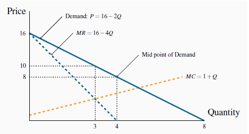
For a linear demand curve the price elasticity has a value of unity ( - 1) at the mid point. Since TR is maximized here it follows that no additional revenue can be generated from further sales; that is, the MR is zero. Profit is maximized where MR = MC, where Q = 3. The price at this output is read from the demand curve: P = 16 - 2.3 = 10.
From Measures of response: elasticities we know that, when the demand curve is a straight line, the midpoint has an elasticity value of unity and also is the point where total revenue is greatest (see Figure 4.4). It follows that, since total revenue is greatest at the midpoint, this point must also define the output where the addition to revenue from further sales goes from positive to negative. That is, the MR curve is zero at the midpoint of the linear demand curve. The MR curve in Figure 10.5 reflects this: the midpoint on the quantity axis is 4 units and therefore MR must be zero at that point.
Furthermore, since theMR intersects the quantity axis at a point half way to the horizontal intercept of the demand curve, it must have a slope that is twice the slope of the demand curve. Hence the MR curve can be written as the demand curve with twice the slope:
MR = 16 - 4Q.
The profit maximum is obtained from the intersection of the MR and the MC. So let us equate these to obtain the optimal output:
MR = MC implies: 16 - 4Q = 1+1Q,
that is,

We have found the profit maximizing output. What price will the monopolist choose? This is obtained from the demand curve. The optimal, or profit maximizing, price is:

Total revenue is therefore $30 (3 _ $10). Total cost can be obtained from the average cost curve, which in this case is ATC = 1+Q/2. At Q = 3, average cost is $2.5 (1 + 3/2). Thus total cost is $7.5 and profit is $22.5. Note that this value differs slightly from the value in Table 10.1 and derived from Figure 10.4, as we would expect, because we use straight line functions rather than step functions and they are not identical 1 .
- 3085 reads
