Discrete-Time Fourier Transform (DTFT)

Available under Creative Commons-ShareAlike 4.0 International License.

The Fourier transform of the discrete-time signal s (n) is defined to be

$S(e^{j2\pi f})=\sum_{n=-\infty }^{\infty }\left ( s(n)e^{-(j2\pi fn)} \right )$

Frequency here has no units. As should be expected, this Definition is linear, with the transform of a sum of signals equaling the sum of their transforms. Real-valued signals have conjugate-symmetric spectra: $S(e^{-(j2\pi f)})=S(e^{j2\pi f})^{*}.$

Exercise 5.6.1

A special property of the discrete-time Fourier transform is that it is periodic with period one: $S\left ( e^{j2\pi (f+1)} \right )=S\left ( e^{j2\pi f} \right ).$

Derive this property from the Definition of the DTFT.

Because of this periodicity, we need only plot the spectrum over one period to understand completely the spectrum's structure; typically, we plot the spectrum over the frequency range $\left [ -\left ( \frac{1}{2} \right ),\frac{1}{2} \right ].$ When the signal is real-valued, we can further simplify our plotting chores by showing the spectrum only over $\left [ 0,\frac{1}{2} \right ];$ the spectrum at negative frequencies can be derived from positive-frequency spectral values. When we obtain the discrete-time signal via sampling an analog signal, the Nyquist frequency (p. 176) corresponds to the discrete-time frequency $\frac{1}{2}.$ To show this, note that a sinusoid having a frequency equal to the Nyquist frequency $\frac{1}{2T_{S}}$ has a sampled waveform that equals

$\cos \left ( 2\pi \times \frac{1}{2Ts}nTs \right )=\cos (\pi n)=(-1)^{n}$

The exponential in the DTFT at frequency $\frac{1}{2}$ equals $e^{-\left ( \frac{j2\pi n}{2} \right )}=e^{-(j\pi n)}=(-1)^{n}$ meaning that discrete-time frequency equals analog frequency multiplied by the sampling interval

f_D = f_AT_s 　　　 (5.18)

f_Dand f_Arepresent discrete-time and analog frequency variables, respectively. The aliasing figure (Figure 5.4) provides another way of deriving this result. As the duration of each pulse in the periodic sampling signal PT_s(t) narrows, the amplitudes of the signal's spectral repetitions, which are governed by the Fourier series coefficients (4.10) of PT_s(t), become increasingly equal. Examination of the periodic pulse signal (Figure 4.1) reveals that as Δ decreases, the value of c₀, the largest Fourier coefficient, decreases to zero: $\left | C_{0} \right |=\frac{A\Delta }{T_{s}}.$ Thus, to maintain a mathematically viable Sampling Theorem, the amplitude A must increase as $\frac{1}{\Delta },$ becoming infinitely large as the pulse duration decreases. Practical systems use a small value of Δ, say 0.1 · T_s and use amplifiers to rescale the signal. Thus, the sampled signal's spectrum becomes periodic with period $\frac{1}{T_{s} }$ . Thus, the Nyquist frequency $\frac{1}{2T_{s} }$ corresponds to the frequency $\frac{1}{2}.$

Example 5.1

Let's compute the discrete-time Fourier transform of the exponentially decaying sequence s(n)=aⁿu(n), where u (n) is the unit-step sequence. Simply plugging the signal's expression into the Fourier transform formula,

$\begin{align*} S(e^{j2\pi f})&=\sum_{n=-\infty }^{\infty }\left ( a^{n}u\left ( n \right )e^{-\left ( j2\pi fn \right )} \right )\\ &= \sum_{n=0}^{\infty }\left ( \left ( ae^{-\left ( j2\pi f \right )} \right )^{n} \right )\\ \end{align*}$

This sum is a special case of the geometric series.

$\sum_{n=0}^{\infty }\left ( a^{n} \right )=\frac{1}{1-\alpha }\:,\ \:\left | \alpha \right |< 1$

Thus, as long as |a| < 1, we have our Fourier transform.

$S(e^{j2\pi f})=\frac{1}{1-ae^{-(j2\pi f)}}^}$

Using Euler's relation, we can express the magnitude and phase of this spectrum.

$\left | s(e^{j2\pi f}) \right |=\frac{1}{\sqrt{(1-a\cos (2\pi f))^{2}+a^{2}\sin ^{2}(2\pi f)}}$

$\angle \left ( S\left ( e^{j2\pi f} \right ) \right )=-\left ( \tan ^{-1}\left ( \frac{a\sin(2\pi f)}{1-a\cos(2\pi f)} \right ) \right )$

No matter what value of a we choose, the above formulae clearly demonstrate the periodic nature of the spectra of discrete-time signals. Figure 5.9 (Spectrum of exponential signal) shows indeed that the spectrum is a periodic function. We need only consider the spectrum between $-\frac{1}{2}$ and $\frac{1}{2}$ to unambiguously define it. When a> 0, we have a lowpass spectrum the spectrum diminishes as frequency increases from 0 to $\frac{1}{2}$ with increasing a leading to a greater low frequency content; for a< 0, we have a highpass spectrum (Figure 5.10 (Spectra of exponential signals)).

Figure 5.9 Spectrum of exponential signall

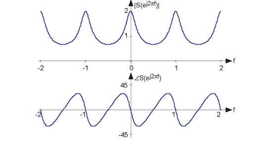
The spectrum of the exponential signal (a = 0:5) is shown over the frequency range [-2,2], clearly demonstrating the periodicity of all discrete-time spectra. The angle has units of degrees.

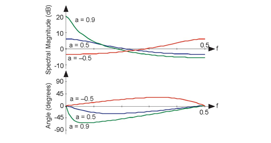
Figure 5.10 Spectra of exponential signals

The spectra of several exponential signals are shown. What is the apparent relationship between the spectra for a = 0.5 and a = -0.5?

Example 5.2

Analogous to the analog pulse signal, let's find the spectrum of the length-N pulse sequence.

$s(n)=\left\{\begin{matrix} 1\:if\:0\leq n\leq N-1\\0\:otherwise \end{matrix}\right.$

(5.24)

The Fourier transform of this sequence has the form of a truncated geometric series.

$S(e^{j2\pi f})=\sum_{n=0}^{N-1}\left ( e^{-(j2\pi fn) \right )}$

(5.25)

For the so-called finite geometric series, we know that

$\sum_{n=n_{0}}^{N+n_{0}-1}\left ( \alpha ^{n} \right )=\alpha ^{n_{0}}\frac{1-\alpha ^{N}}{1-\alpha }$

(5.26)

for all values of α.

Exercise 5.6.2

Derive this formula for the finite geometric series sum. The "trick" is to consider the difference between the series' sum and the sum of the series multiplied by α. Applying this result yields (Figure 5.11 (Spectrum of length-ten pulse).)

$\begin{align*} S(e^{j2\pi f})&=\frac{1-e^{-(j2\pi fN)}}{1-e^{-(j2\pi f)}}\\ &=e^{-(j\pi f(N-1))}\frac{\sin(\pi fN)}{\sin(\pi f)} \\ \end{align*}$

The ratio of sine functions has the generic form of $\frac{\sin(Nx)}{\sin(x)},$ which is known as the discrete-time sinc function dsinc (x). Thus, our transform can be concisely expressed as $S\left ( e^{j2\pi f} \right )=e^{-(j\pi f(N-1))} dsinc (\pi f),$ The discrete-time pulse's spectrum contains many ripples, the number of which increase with N, the pulse's duration.

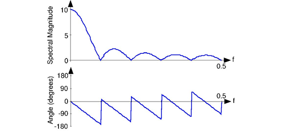
Figure 5.11 Spectrum of length-ten pulse

The spectrum of a length-ten pulse is shown. Can you explain the rather complicated appearance of the phase?

The inverse discrete-time Fourier transform is easily derived from the following relationship:

$\int_{-\left ( \frac{1}{2} \right )}^{\frac{1}{2}}e^{-(j2\pi fm)}e^{j2\pi fn}df=\left\{\begin{matrix} 1\: if\: m=n\\ 0\: if\: m\neq n \end{matrix}$

Therefore, we find that

$\begin{align*} \int_{-\left ( \frac{1}{2} \right )}^{\frac{1}{2}}S(e^{j2\pi f})e^{j2\pi fn}df &= \int_{-\left ( \frac{1}{2} \right )}^{\frac{1}{2}}\sum _{m}\left ( s(m)e^{-(j2\pi fm)}e^{j2\pi fn} \right )df \\ &= \sum_{m}\left ( s\left ( m \right )\int_{-\left ( \frac{1}{2} \right )}^{\frac{1}{2}}e^{\left ( -\left ( j2\pi f \right ) \right )\left ( m-n \right )}df \right )\\ &=s\left ( n \right )\\ \end{align*}$

The Fourier transform pairs in discrete-time are

$S(e^{j2\pi f})=\sum_{n=-\infty }^{\infty }\left ( s(n)e^{-(j2\pi fn) \right )}$

$s(n)=\int_{-\left ( \frac{1}{2} \right )}^{\frac{1}{2}}S(e^{j2\pi f})e^{j2\pi fn}df$

The properties of the discrete-time Fourier transform mirror those of the analog Fourier transform. The DTFT properties table shows similarities and diferences. One important common property is Parseval's Theorem.

$\sum_{n=-\infty }^{\infty }\left ( (\left | s(n) \right |)^{2} \right )=\int_{-\left ( \frac{1}{2} \right )}^{\frac{1}{2}}\left ( \left | S(e^{j2\pi f} \right ) \right |)^{2}df$

To show this important property, we simply substitute the Fourier transform expression into the frequency-domain expression for power.

$\begin{align*} \int_{-\left ( \frac{1}{2} \right )}^{\frac{1}{2}}(\left | S(e^{j2\pi f}) \right |)^{2}df &=\int_{-\left ( \frac{1}{2} \right )}^{\frac{1}{2}}\left ( \sum_{n}\left ( s(n)e^{-(j2\pi fn)} \right ) \right )\sum_{m}\left ( s(n)^{*}e^{j2\pi fm} \right )df \\ &=\sum _{n,m}\left ( s(n)s(n)^{*}\int_{-\left ( \frac{1}{2} \right )}^{\frac{1}{2}}e^{j2\pi f(m-n)}df \right )\\ \end{align*}$

Using the orthogonality relation (5.28), the integral equals δ (m − n), where δ (n) is the unit sample (Figure 5.8: Unit sample). Thus, the double sum collapses into a single sum because nonzero values occur only when n = m, giving Parseval's Theorem as a result. We term $\sum _{n}\left ( s^{2}(n) \right )$ the energy in the discrete-time signal s(n) in spite of the fact that discrete-time signals don't consume (or produce for that matter) energy. This terminology is a carry-over from the analog world.

Exercise 5.6.3

Suppose we obtained our discrete-time signal from values of the product s(t)p_Ts(t), where the duration of the component pulses in p_Ts(t) is Δ. How is the discrete-time signal energy related to the total energy contained in s(t)? Assume the signal is bandlimited and that the sampling rate was chosen appropriate to the Sampling Theorem's conditions.

瀏覽次數：3665

您在這裡

Discrete-Time Fourier Transform (DTFT)