Solutions to Exercises in Chapter 6

Available under Creative Commons-ShareAlike 4.0 International License.

Solution to Exercise 6.3.1

In both cases, the answer depends less on geometry than on material properties. For coaxial cable,

$c=\frac{1}{\sqrt{\mu _{d}\epsilon _{d}}}.$

For twisted pair,

$c=\frac{1}{\sqrt{\mu \epsilon }}\sqrt{\frac{arccosh(\frac{d}{2r})}{\frac{\delta }{2r}+arccosh\left (\frac{d}{2r} \right )}}.$

Solution to Exercise 6.3.2

You can find these frequencies from the spectrum allocation chart (Frequency Allocations). Light in the middle of the visible band has a wavelength of about 600 nm, which corresponds to a frequency of 5 × 10₁₄Hz . Cable television transmits within the same frequency band as broadcast television (about 200 MHz or 2 × 10⁸Hz ). Thus, the visible electromagnetic frequencies are over six orders of magnitude higher!

Solution to Exercise 6.3.3

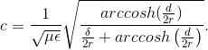
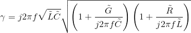
As frequency increases,

$\left ( 2\pi f \tilde{C}\gg \tilde{G} \right )$

and

$\left ( 2\pi f \tilde{L}\gg \tilde{R} \right ).$

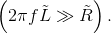
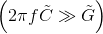
In this high-frequency region,

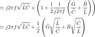
$\gamma =j2\pi f \sqrt{\tilde{L}\tilde{C}}\sqrt{\left ( 1+\frac{\tilde{G}}{j2\pi f \tilde{C}} \right )\left ( 1+\frac{\tilde{R}}{j2\pi f \tilde{L}} \right )}$
$\begin{align*}&\simeq j2\pi f \sqrt{\tilde{L}\tilde{C}} \times \left (1+\frac{1}{2}\frac{1}{j2\pi f} \left (\frac{\tilde{G}}{\tilde{C}}+\frac{\tilde{R}}{\tilde{L}} \right ) \right )\\&\simeq j2\pi f \sqrt{\tilde{L}\tilde{C}} + \frac{1}{2} \left (\tilde{G}\sqrt{\frac{\tilde{L}}{\tilde{C}}}+\tilde{R}\sqrt{\frac{\tilde{C}}{\tilde{L}}} \right )\\ \end{align*}$

(6.65)

Thus, the attenuation (space) constant equals the real part of this expression, and equals

$a(f)=\frac{\tilde{G}Z_{0}+\frac{\tilde{R}}{Z_{0}}}{2}.$

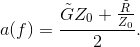
Solution to Exercise 6.4.1

As shown previously (Modulated Communication), voltages and currents in a wireline channel, which is modeled as a transmission line having resistance, capacitance and inductance, decay exponentially with distance. The inverse-square law governs free-space propagation because such propagation is lossless, with the inverse-square law a consequence of the conservation of power. The exponential decay of wireline channels occurs because they have losses and some filtering.

Solution to Exercise 6.5.1

Figure 6.43 Figure 6.43

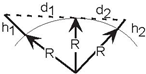
Use the Pythagorean Theorem, (h + R)² = R² + d², where h is the antenna height, d is the distance from the top of the earth to a tangency point with the earth's surface, and R the earth's radius. The line-of-sight distance between two earth-based antennae equals

$d_{LOS}=\sqrt{2h_{1}R+h{_{1}}^{2}}+\sqrt{2h_{2}R+h{_{2}}^{2}}$

As the earth's radius is much larger than the antenna height, we have to a good approximation that

$d_{LOS}=\sqrt{2h_{1}R}+\sqrt{2h_{2}R}.$

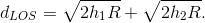
If one antenna is at ground elevation, say h₂ =0 , the other antenna's range is

$\sqrt{2h_{1}R}.$

Solution to Exercise 6.5.2

As frequency decreases, wavelength increases and can approach the distance between the earth's surface and the ionosphere. Assuming a distance between the two of 80 km, the relation λf = c gives a corresponding frequency of 3.75 kHz. Such low carrier frequencies would be limited to low bandwidth analog communication and to low datarate digital communications. The US Navy did use such a communication scheme to reach all of its submarines at once.

Solution to Exercise 6.7.1

Transmission to the satellite, known as the uplink, encounters inverse-square law power losses. Reflecting of the ionosphere not only encounters the same loss, but twice. Refection is the same as transmitting exactly what arrives, which means that the total loss is the product of the uplink and downlink losses. The geosynchronous orbit lies at an altitude of 35700km. The ionosphere begins at an altitude of about 50 km. The amplitude loss in the satellite case is proportional to 2.8 × 10⁻⁸; for Marconi, it was proportional to 4.4 × 10⁻¹⁰. Marconi was very lucky.

Solution to Exercise 6.8.1

If the interferer's spectrum does not overlap that of our communications channel - the interferer is out-of-band we need only use a bandpass filter that selects our transmission band and removes other portions of the spectrum.

Solution to Exercise 6.9.1

The additive-noise channel is not linear because it does not have the zero-input-zero-output property (even though we might transmit nothing, the receiver's input consists of noise).

Solution to Exercise 6.11.1

The signal-related portion of the transmitted spectrum is given by

$X(f)=\frac{1}{2}M(f-f_{c})+\frac{1}{2}M(f+f_{c}).$

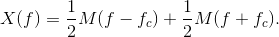
Multiplying at the receiver by the carrier shifts this spectrum to f_c and to −f_c, and scales the result by half.

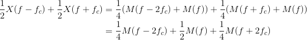
$\begin{align*}\frac{1}{2}X(f-f_{c})+\frac{1}{2}X(f+f_{c})&=\frac{1}{4}(M(f-2f_{c})+M(f))+\frac{1}{4}(M(f+f_{c})+M(f))\\ &= \frac{1}{4}M(f-2f_{c})+\frac{1}{2}M(f)+\frac{1}{4}M(f+2f_{c})\\ \end{align*}$

(6.67)

The signal components centered at twice the carrier frequency are removed by the lowpass filter, while the baseband signal M(f) emerges.

Solution to Exercise 6.12.1

The key here is that the two spectra M (f − f_c), M (f + f_c) do not overlap because we have assumed that the carrier frequency fc is much greater than the signal's highest frequency. Consequently, the term M (f − f_c) M (f + f_c) normally obtained in computing the magnitude-squared equals zero.

Solution to Exercise 6.12.2

Separation is 2W. Commercial AM signal bandwidth is 5 kHz. Speech is well contained in this bandwidth, much better than in the telephone!

Solution to Exercise 6.13.1

$x(t)=\sum_{n=-\infty }^{\infty }\left ( s_{b(n)}(t-nT) \right ).$

Solution to Exercise 6.14.1

k =4.

Solution to Exercise 6.14.2

$x(t)=\sum _{n}\left ( (-1)^{b(n)}Ap_{T}(t-nT)\sin\left ( \frac{2\pi kt}{T} \right ) \right )$

Solution to Exercise 6.14.3

The harmonic distortion is 10%.

Solution to Exercise 6.14.4

Twice the baseband bandwidth because both positive and negative frequencies are shifted to the carrier by the modulation: 3R.

Solution to Exercise 6.16.1

In BPSK, the signals are negatives of each other: s₁ (t)= −s₀ (t). Consequently, the output of each multiplier-integrator combination is the negative of the other. Choosing the largest therefore amounts to choosing which one is positive. We only need to calculate one of these. If it is positive, we are done. If it is negative, we choose the other signal.

Solution to Exercise 6.16.2

The matched filter outputs are $\pm \left ( \frac{A^{2}T}{2} \right )$

because the sinusoid has less power than a pulse having the same amplitude.

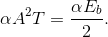
Solution to Exercise 6.17.1

The noise-free integrator outputs differ by αA²T , the factor of two smaller value than in the baseband case arising because the sinusoidal signals have less energy for the same amplitude. Stated in terms of E_b, the difference equals 2αE_b just as in the baseband case.

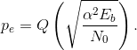
Solution to Exercise 6.18.1

The noise-free integrator output difference now equals

$\alpha A^{2}T=\frac{\alpha E_{b}}{2}.$

The noise power remains the same as in the BPSK case, which from the probability of error equation (6.46) yields

$p_{e}=Q\left ( \sqrt{\frac{\alpha ^{2}E_{b}}{N_{0}}} \right ).$

Solution to Exercise 6.20.1

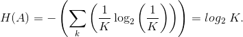Equally likely symbols each have a probability of $\frac{1}{K}.$ Thus, $H(A)=-\left ( \sum _{k}\left ( \frac{1}{K}\log_{2}\left ( \frac{1}{K} \right ) \right ) \right )=log_{2}\ K.$ To prove that this is the maximum-entropy probability assignment, we must explicitly take into account that probabilities sum to one. Focus on a particular symbol, say the first. Pr [a₀] appears twice in the entropy formula: the terms Pr[a₀] log₂Pr[a₀]and (1 −Pr[a₀]+ ··· + Pr[a_K₋₂]) log₂(1 −Pr [a₀]+ ··· + Pr [a_K₋₂]) . The derivative with respect to this probability (and all the others) must be zero. The derivative equals log₂Pr [a₀] − log₂ (1 −Pr [a₀]+ ··· + Pr[a_K₋₂]), and all other derivatives have the same form (just substitute your letter's index). Thus, each probability must equal the others, and we are done. For the minimum entropy answer, one term is 1log₂1=0 , and the others are 0log₂0 , which we define to be zero also. The minimum value of entropy is zero.

Solution to Exercise 6.22.1

The Huffman coding tree for the second set of probabilities is identical to that for the first (Figure 6.18 (Huffman Coding Tree)). The average code length is 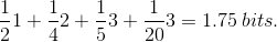$\frac{1}{2}1+\frac{1}{4}2+\frac{1}{5}3+\frac{1}{20}3=1.75\:bits.$ The entropy calculation 2 4 5 20 is straightforward: $H(A)=-\left ( \frac{1}{2}\log\left ( \frac{1}{2} \right )+\frac{1}{4}\log\left ( \frac{1}{4} \right )+\frac{1}{5}\left \log \left ( \frac{1}{5} \right )+\frac{1}{20}\log\left ( \frac{1}{20} \right ) \right ).$ which equals 1.68 bits.

Solution to Exercise 6.23.1

$T=\frac{1}{\bar {B(A)}R}.$

Solution to Exercise 6.23.2

Because no codeword begins with another's codeword, the first codeword encountered in a bit stream must be the right one. Note that we must start at the beginning of the bit stream; jumping into the middle does not guarantee perfect decoding. The end of one codeword and the beginning of another could be a codeword, and we would get lost.

Solution to Exercise 6.23.3

Consider the bitstream ...0110111... taken from the bitstream 0I10I110I110I111I.... We would decode the initial part incorrectly, then would synchronize. If we had a fxed-length code (say 00,01,10,11), the situation is much worse. Jumping into the middle leads to no synchronization at all!

Solution to Exercise 6.25.1

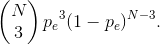
This question is equivalent to 3p_e×(1 − p_e)+p_e²≤ 1 or 2p_e²−3p_e +1 ≥ 0. Because this is an upward-going parabola, we need only check where its roots are. Using the quadratic formula, we find that they are located at $\frac{1}{2}$ and 1. Consequently in the range $0\leq p_{e}\leq \frac{1}{2}$ the error rate produced by coding is smaller.

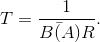
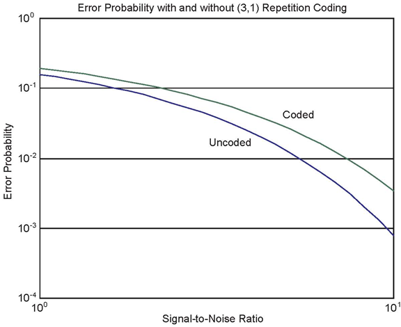
Solution to Exercise 6.26.1

With no coding, the average bit-error probability p_e is given by the probability of error equation (6.47):

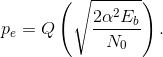
$p_{e}=Q\left (\sqrt{\frac{2\alpha ^{2}E_{b}}{N_{0}}} \right ).$

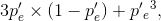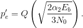With a threefold repetition code, the bit-error probability is given by $3{p}'_{e} \times (1-{p}'_{e})+{p}'{_{e}}^{3},$ where ${p}'_{e} = Q\left (\sqrt{\frac{2\alpha _{2}E_{b}}{3N_{0}}} \right ).$ Plotting this reveals that the increase in bit-error probability out of the channel because of the energy reduction is not compensated by the repetition coding.

Figure 6.44 Error Probability with and without (3,1) Repetition Coding

Solution to Exercise 6.27.1

In binary arithmetic (see 6.27 No Title Provided), adding 0 to a binary value results in that binary value while adding 1 results in the opposite binary value.

Solution to Exercise 6.27.2

d_min=2n +1

Solution to Exercise 6.28.1

When we multiply the parity-check matrix times any codeword equal to a column of G, the result consists of the sum of an entry from the lower portion of G and itself that, by the laws of binary arithmetic, is always zero.

Because the code is linear - sum of any two codewords is a codeword - we can generate all codewords as sums of columns of G. Since multiplying by H is also linear, Hc = 0.

Solution to Exercise 6.28.2

In binary arithmetic see this table, adding 0 to a binary value results in that binary value while adding 1 results in the opposite binary value.

Solution to Exercise 6.28.3

The probability of a single-bit error in a length-N block is Np_e(1 − p_e)^N-1and a triple-bit error has probability

$\left ( \begin{matrix} N\\3 \end{matrix} \right )p{_{e}}^{3}(1-p_{e})^{N-3}.$

For the first to be greater than the second, we must have

$p_{e}< \frac{1}{\sqrt{\frac{(N-1)(N-2)}{6}}+1}$

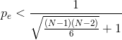
For N =7, p_e< 0.31.

Solution to Exercise 6.29.1

In a length-N block, N single-bit and $\frac{N(N-1)}{2}$ double-bit errors can occur. The number of non-zero vectors resulting from $H\hat{c}$ must equal or exceed the sum of these two numbers.

$2^{N-K}-1\geq N+\frac{N(N-1)}{2}or\;2^{N-K}\geq \frac{N_{2}+N+2}{2}$

(6.68)

The first two solutions that attain equality are (5,1) and (90,78) codes. However, no perfect code exists other than the single-bit error correcting Hamming code. (Perfect codes satisfy relations like (6.68) with equality.)

Solution to Exercise 6.31.1

To convert to bits/second, we divide the capacity stated in bits/transmission by the bit interval duration T.

Solution to Exercise 6.33.1

The network entry point is the telephone handset, which connects you to the nearest station. Dialing the telephone number informs the network of who will be the message recipient. The telephone system forms an electrical circuit between your handset and your friend's handset. Your friend receives the message via the same device the handset that served as the network entry point.

Solution to Exercise 6.36.1

The transmitting op-amp sees a load or 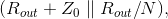$(R_{out} + Z_{0} \parallel R_{out}/N),$ where N is the number of transceivers other than this one attached to the coaxial cable. The transfer function to some other transceiver's receiver circuit is Rout divided by this load.

Solution to Exercise 6.36.2

The worst-case situation occurs when one computer begins to transmit just before the other's packet arrives. Transmitters must sense a collision before packet transmission ends. The time taken for one computer's packet to travel the Ethernet's length and for the other computer's transmission to arrive equals the round-trip, not one-way, propagation time.

Solution to Exercise 6.36.3

The cable must be a factor of ten shorter: It cannot exceed 100 m. Different minimum packet sizes means different packet formats, making connecting old and new systems together more complex than need be.

Solution to Exercise 6.37.1

When you pick up the telephone, you initiate a dialog with your network interface by dialing the number. The network looks up where the destination corresponding to that number is located, and routes the call accordingly. The route remains fixed as long as the call persists. What you say amounts to high-level protocol while establishing the connection and maintaining it corresponds to low-level protocol.

瀏覽次數：6270

您在這裡

Solutions to Exercises in Chapter 6