Discrete-Time Systems in the Time-Domain

Available under Creative Commons-ShareAlike 4.0 International License.

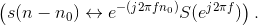
A discrete-time signal s(n) is delayed by n₀ samples when we write s(n - n₀), with n₀ > 0. Choosing n₀ to be negative advances the signal along the integers. As opposed to analog delays (Delay : Delay), discrete-time delays can only be integer valued. In the frequency domain, delaying a signal corresponds to a linear phase shift of the signal's discrete-time Fourier transform :

Linear discrete-time systems have the superposition property.

(5.40)

A discrete-time system is called shift-invariant (analogous to time-invariant analog systems (Time-Invariant Systems ) if delaying the input delays the corresponding output. If S (x (n)) = y (n), then a shift-invariant system has the property

(5.41)

We use the term shift-invariant to emphasize that delays can only have integer values in discrete-time, while in analog signals, delays can be arbitrarily valued.

We want to concentrate on systems that are both linear and shift-invariant. It will be these that allow us the full power of frequency-domain analysis and implementations. Because we have no physical constraints in "constructing" such systems, we need only a mathematical specification. In analog systems, the differential equation specifies the input-output relationship in the time-domain. The corresponding discrete-time specification is the difference equation.

(5.42)

Here, the output signal y (n) is related to its past values y (n - l), l = {1; … ; p}, and to the current and past values of the input signal x (n). The system's characteristics are determined by the choices for the number of coefficients p and q and the coefficients' values {a₁, ... , a_p} and {b₀, b₁, ... , b_q}.

ASIDE: There is an asymmetry in the coefficients: where is a₀? This coefficient would multiply the y(n) term in (5.42). We have essentially divided the equation by it, which does not change the input-output relationship. We have thus created the convention that a₀ is always one.

As opposed to differential equations, which only provide an implicit description of a system (we must somehow solve the differential equation), difference equations provide an explicit way of computing the output for any input. We simply express the difference equation by a program that calculates each output from the previous output values, and the current and previous inputs.

Difference equations are usually expressed in software with for loops. A MATLAB program that would compute the first 1000 values of the output has the form

for n=1:1000
    y(n) = sum(a.*y(n-1:-1:n-p)) + sum(b.*x(n:-1:n-q));
end

An important detail emerges when we consider making this program work; in fact, as written it has (at least) two bugs. What input and output values enter into the computation of y (1)? We need values for y (0), y (−1), ..., values we have not yet computed. To compute them, we would need more previous values of the output, which we have not yet computed. To compute these values, we would need even earlier values, ad infinitum. The way out of this predicament is to specify the system's initial conditions: we must provide the p output values that occurred before the input started. These values can be arbitrary, but the choice does impact how the system responds to a given input. One choice gives rise to a linear system: Make the initial conditions zero. The reason lies in the Definition of a linear system (Section 2.6.6: Linear Systems): The only way that the output to a sum of signals can be the sum of the individual outputs occurs when the initial conditions in each case are zero.

Exercise 5.12.1

The initial condition issue resolves making sense of the difference equation for inputs that start at some index. However, the program will not work because of a programming, not conceptual, error. What is it? How can it be "fixed?"

Example 5.5

Let's consider the simple system having p =1 and q =0.

(5.43)

To compute the output at some index, this difference equation says we need to know what the previous output y (n − 1) and what the input signal is at that moment of time. In more detail, let's compute this system's output to a unit-sample input: x (n)= δ (n). Because the input is zero for negative indices, we start by trying to compute the output at n = 0.

(5.44)

What is the value of y (−1)? Because we have used an input that is zero for all negative indices, it is reasonable to assume that the output is also zero. Certainly, the difference equation would not describe a linear system (Section 2.6.6: Linear Systems) if the input that is zero for all time did not produce a zero output. With this assumption, y (−1) = 0, leaving y (0) = b. For n> 0, the input unit-sample is zero, which leaves us with the difference equation y (n)= ay (n − 1) , n> 0 . We can envision how the filter responds to this input by making a table.

 　 　 　 (5.45)

Coefficient values determine how the output behaves. The parameter b can be any value, and serves as a gain. The effect of the parameter a is more complicated (Table). If it equals zero, the output simply equals the input times the gain b. For all non-zero values of a, the output lasts forever; such systems are said to be IIR (Infinite Impulse Response). The reason for this terminology is that the unit sample also known as the impulse (especially in analog situations), and the system's response to the "impulse" lasts forever. If a is positive and less than one, the output is a decaying exponential. When a =1, the output is a unit step. If a is negative and greater than −1, the output oscillates while decaying exponentially. When a = −1, the output changes sign forever, alternating between b and −b. More dramatic effects when |a| > 1; whether positive or negative, the output signal becomes larger and larger, growing exponentially.

Figure 5.18

 

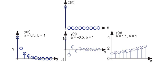
The input to the simple example system, a unit sample, is shown at the top, with the outputs for several system parameter values shown below. 

Positive values of a are used in population models to describe how population size increases over time. Here, n might correspond to generation. The diference equation says that the number in the next generation is some multiple of the previous one. If this multiple is less than one, the population becomes extinct; if greater than one, the population fourishes. The same diference equation also describes the effect of compound interest on deposits. Here, n indexes the times at which compounding occurs (daily, monthly, etc.), a equals the compound interest rate plus one, and b =1 (the bank provides no gain). In signal processing applications, we typically require that the output remain bounded for any input. For our example, that means that we restrict |a| < 1 and choose values for it and the gain according to the application.

Exercise 5.12.2

Note that the difference equation (5.42),

does not involve terms like y (n + 1) or x (n + 1) on the equation's right side. Can such terms also be included? Why or why not?

Figure 5.19 The plot shows the unit-sample response of a length-5 boxcar filter.

 

Example 5.6

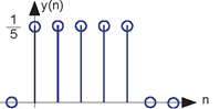
A somewhat different system has no "a" coefficients. Consider the difference equation

(5.46)

Because this system's output depends only on current and previous input values, we need not be concerned with initial conditions. When the input is a unit-sample, the output equals  for n = {0,...,q − 1}, then equals zero thereafter. Such systems are said to be FIR (Finite Impulse Response) because their unit sample responses have finite duration. Plotting this response (Figure 5.19) shows that the unit-sample response is a pulse of width q and height This waveform is also known as a boxcar, hence the name boxcar filter given to this system. 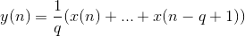We'll derive its frequency response and develop its filtering interpretation in the next section. For now, note that the difference equation says that each output value equals the average of the input's current and previous values. Thus, the output equals the running average of input's previous q values. Such a system could be used to produce the average weekly temperature (q =7) that could be updated daily.

[MEDIA OBJECT]