


One wonders if the DFT can be computed faster: Does another computational procedure an algorithm exist that can compute the same quantity, but more efficiently. We could seek methods that reduce the constant of proportionality, but do not change the DFT's complexity O(N2). Here, we have something more dramatic in mind: Can the computations be restructured so that a smaller complexity results?
In 1965, IBM researcher Jim Cooley and Princeton faculty member John Tukey developed what is now known as the Fast Fourier Transform (FFT). It is an algorithm for computing that DFT that has order O(NlogN) for certain length inputs. Now when the length of data doubles, the spectral computational time will not quadruple as with the DFT algorithm; instead, it approximately doubles. Later research showed that no algorithm for computing the DFT could have a smaller complexity than the FFT. Surprisingly, historical work has shown that Gauss2l in the early nineteenth century developed the same algorithm, but did not publish it! After the FFT's rediscovery, not only was the computation of a signal's spectrum greatly speeded, but also the added feature of algorithm meant that computations had flexibility not available to analog implementations.
Exercise 5.9.1
Before developing the FFT, let's try to appreciate the algorithm's impact. Suppose a short-length transform takes 1 ms. We want to calculate a transform of a signal that is 10 times longer. Compare how much longer a straightforward implementation of the DFT would take in comparison to an FFT, both of which compute exactly the same quantity.
To derive the FFT, we assume that the signal's duration is a power of two: N=2L. Consider what happens to the even-numbered and odd-numbered elements of the sequence in the DFT calculation.
![\begin{align*} S(k)&=s(0)+s(2)e^{(-j)\frac{2\pi 2k}{N}}+...+s(N-2)e^{\left ( -j \right )\frac{2\pi (N-2)k}{N}}\\ &\ \ \ +s(1)e^{(-j)\frac{2\pi k}{N}}+s(3)e^{(-j)\frac{2\pi (2+1)k}{N}}+\cdots +s\left ( N-1 \right )e^{(-j)\frac{2\pi (N-(2-1))k}{N}}\\ &=\left [ s(0)+s(2)e^{(-j)\frac{2\pi k}{\frac{N}{2}}} +...+s(N-2)e^{(-j)\frac{2\pi \left ( \frac{N}{2}-1 \right )k}{\frac{N}{2}}}\right ]\\ &\ \ \ +\begin{bmatrix} s(1)+s(3)e^{(-j)\frac{2}{\pi }}+...+s(N-1)e^{(-j)\frac{2\pi \left ( \frac{N}{2}-1 \right )}{\frac{N}{2}}} \end{bmatrix}e\frac{-\left ( j2\pi k \right )}{N}\\ \end{align*}](/system/files/resource/9/9648/9758/media/eqn-img_26.gif)
(5.39)
Each term in square brackets has the form of a  DFT. The
first one is a DFT of the even-numbered elements, and the second of the odd-numbered elements. The first DFT is combined with the second multiplied by the complex exponential
DFT. The
first one is a DFT of the even-numbered elements, and the second of the odd-numbered elements. The first DFT is combined with the second multiplied by the complex exponential  The half-length transforms are each evaluated at
frequency indices k = 0, ..., N - 1. Normally, the number of frequency indices in a DFT calculation range between zero and the transform length minus one. The computational advantage of the FFT comes from recognizing the periodic nature of the discrete Fourier transform. The FFT simply reuses the computations made in the half-length
transforms and combines them through additions and the multiplication by e, which is not periodic over
The half-length transforms are each evaluated at
frequency indices k = 0, ..., N - 1. Normally, the number of frequency indices in a DFT calculation range between zero and the transform length minus one. The computational advantage of the FFT comes from recognizing the periodic nature of the discrete Fourier transform. The FFT simply reuses the computations made in the half-length
transforms and combines them through additions and the multiplication by e, which is not periodic over  Figure 5.12 (Length-8 DFT decomposition) illustrates this decomposition. As it stands, we now compute
transforms  multiply one of them by the complex
exponential (complexity O(N)), and add the results (complexity O(N)). At this point, the total complexity is still dominated by the half-length DFT calculations, but the
proportionality coefficient has been reduced.
multiply one of them by the complex
exponential (complexity O(N)), and add the results (complexity O(N)). At this point, the total complexity is still dominated by the half-length DFT calculations, but the
proportionality coefficient has been reduced.
Now for the fun. Because N=2L, each of the half-length transforms can be reduced to two quarter-length transforms, each of these to two eighth-length ones, etc. This
decomposition continues until we are left with length-2 transforms. This transform is quite simple, involving only additions. Thus, the first stage of the FFT has  length-2 transforms (see the bottom part of Figure 5.12 (Length-8 DFT decomposition)). Pairs of these transforms are combined by
adding one to the other multiplied by a complex exponential. Each pair requires 4 additions and 2 multiplications, giving a total number of computations equaling
length-2 transforms (see the bottom part of Figure 5.12 (Length-8 DFT decomposition)). Pairs of these transforms are combined by
adding one to the other multiplied by a complex exponential. Each pair requires 4 additions and 2 multiplications, giving a total number of computations equaling  This number of computations does not change from stage to stage.
Because the number of stages, the number of times the length can be divided by two, equals log2N, the number of arithmetic operations equals
This number of computations does not change from stage to stage.
Because the number of stages, the number of times the length can be divided by two, equals log2N, the number of arithmetic operations equals  which makes the complexity of the FFT
O(Nlog2N).
which makes the complexity of the FFT
O(Nlog2N).
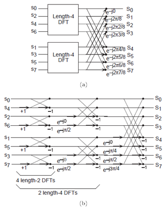
Doing an example will make computational savings more obvious. Let's look at the details of a length-8 DFT. As shown on Figure 5.13 (Butterfy), we first decompose the DFT into two length-4 DFTs, with the outputs added and subtracted together in pairs. Considering Figure 5.13 (Butterfy) as the frequency index goes from 0 through 7, we recycle values from the length-4 DFTs into the fnal calculation because of the periodicity of the DFT output. Examining how pairs of outputs are collected together, we create the basic computational element known as a butterfy (Figure 5.13 (Butterfy)).
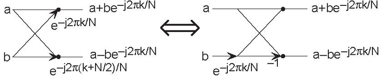
The basic computational element of the fast Fourier transform is the butterfly. It takes two complex numbers, represented by a and b, and forms the quantities shown. Each butterfly requires one complex multiplication and two complex additions.
By considering together the computations involving common output frequencies from the two half-length DFTs, we see that the two complex multiplies are related to each other, and we can reduce
our computational work even further. By further decomposing the length-4 DFTs into two length-2 DFTs and combining their outputs, we arrive at the diagram summarizing the length-8 fast Fourier
transform (Figure 5.12 (Length-8 DFT
decomposition)). Although most of the complex multiplies are quite simple (multiplying by  means swapping real and imaginary parts and changing their signs), let's count those for purposes of evaluating the complexity as
full complex multiplies. We have
means swapping real and imaginary parts and changing their signs), let's count those for purposes of evaluating the complexity as
full complex multiplies. We have  complex multiplies and
N =8 complex additions for each stage and log2N = 3 stages, making the number of basic computations
complex multiplies and
N =8 complex additions for each stage and log2N = 3 stages, making the number of basic computations  as predicted.
Exercise 5.9.2
Note that the ordering of the input sequence in the two parts of Figure 5.12 (Length-8 DFT decomposition) aren't quite the same. Why not? How is the ordering determined?
Other "fast" algorithms were discovered, all of which make use of how many common factors the transform length N has. In number theory, the number of prime factors a given integer has measures how composite it is. The numbers 16 and 81 are highly composite (equaling 24 and 34 respectively), the number 18 is less so (21 · 32), and 17 not at all (it's prime). In over thirty years of Fourier transform algorithm development, the original Cooley-Tukey algorithm is far and away the most frequently used. It is so computationally efficient that power-of-two transform lengths are frequently used regardless of what the actual length of the data.
Exercise 5.9.3
Suppose the length of the signal were 500? How would you compute the spectrum of this signal using the Cooley-Tukey algorithm? What would the length N of the transform be?
- 瀏覽次數:4093
