


For the (7,4) example, we have 2N-K − 1=7 error patterns that can be corrected. We start with single-bit error patterns, and multiply them by the parity check matrix. If we obtain unique answers, we are done; if two or more error patterns yield the same result, we can try double-bit error patterns. In our case, single-bit error patterns give a unique result.
|
e |
He |
|
1000000 |
101 |
|
0100000 |
111 |
|
0010000 |
110 |
|
0001000 |
011 |
|
0000100 |
100 |
|
0000010 |
010 |
|
0000001 |
001 |
Table 6.3
This corresponds to our decoding table: We associate the parity check matrix multiplication result with the error pattern and add this to the received word. If more than one error occurs (unlikely though it may be), this "error correction" strategy usually makes the error worse in the sense that more bits are changed from what was transmitted.
As with the repetition code, we must question whether our (7,4) code's error correction capability compensates for the increased error probability due to the necessitated reduction in bit energy. Figure 6.23 (Probability of error occurring) shows that if the signal-to-noise ratio is large enough channel coding yields a smaller error probability. Because the bit stream emerging from the source decoder is segmented into four-bit blocks, the fair way of comparing coded and uncoded transmission is to compute the probability of block error: the probability that any bit in a block remains in error despite error correction and regardless of whether the error occurs in the data or in coding buts. Clearly, our (7,4) channel code does yield smaller error rates, and is worth the additional systems required to make it work.
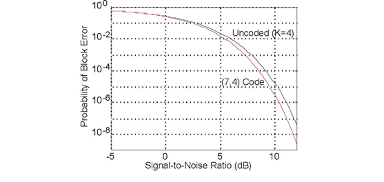
The probability of an error
occurring in transmitted K =4 data bits equals 1 − (1 − pe)4 as (1 − pe)4 equals the probability that the four bits
are received without error. The upper curve displays how this probability of an error anywhere in the four-bit block varies with the signal-to-noise ratio. When a (7,4) single-bit error
correcting code is used, the transmitter reduced the energy it expends during a single-bit transmission by 4/7, appending three extra bits for error correction. Now the probability of any bit
in the seven-bit block being in error after error correction equals  where p'e is the probability of a bit error occurring in the channel when channel coding occurs. Here
 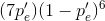 equals the probability of exactly on in seven bits emerging from the
channel in error; The channel decoder corrects this type of error, and all data bits in the block are received correctly.
equals the probability of exactly on in seven bits emerging from the
channel in error; The channel decoder corrects this type of error, and all data bits in the block are received correctly.
Note that our (7,4) code has the length and number of data bits that perfectly fts correcting single bit errors. This pleasant property arises because the number of error patterns that can be corrected, 2N−K − 1, equals the codeword length N. Codes that have 2N−K − 1= N are known as Hamming codes, and the following table (Table 6.3: Hamming Codes) provides the parameters of these codes. Hamming codes are the simplest single-bit error correction codes, and the generator/parity check matrix formalism for channel coding and decoding works for them.
|
N |
K |
E (efficiency) |
|
3 |
1 |
0.33 |
|
7 |
4 |
0.57 |
|
15 |
11 |
0.73 |
|
31 |
26 |
0.84 |
|
63 |
57 |
0.90 |
|
127 |
120 |
0.94 |
Unfortunately, for such large blocks, the probability of multiple-bit errors can exceed the number of single-bit errors unless the channel single-bit error probability Pe is very small. Consequently, we need to enhance the code's error correcting capability by adding double as well as single-bit error correction.
Exercise 6.29.1
What must the relation between N and K be for a code to correct all single-and double-bit errors with a "perfect fit"?
- 瀏覽次數:5063
