


When we incorporate additive noise into our channel model, so that r(t)=αsi(t)+n(t), errors can creep in. If the transmitter sent bit 0 using a BPSK signal set (Section 6.14), the integrators' outputs in the matched filter receiver (Figure 6.14: Optimal receiver structure) would be:
(6.45)
It is the quantities containing the noise terms that cause errors in the receiver's decision-making process. Because they involve noise, the values of these integrals are random quantities drawn from some probability distribution that vary erratically from bit interval to bit interval. Because the noise has zero average value and has an equal amount of power in all frequency bands, the values of the integrals will hover about zero. What is important is how much they vary. If the noise is such that its integral term is more negative than αA2T, then the receiver will make an error, deciding that the transmitted zero-valued bit was indeed a one. The probability that this situation occurs depends on three factors:
- Signal Set Choice - The difference between the signal-dependent terms in the integrators' outputs (equations (6.45)) defines how large the noise term must be for an incorrect receiver decision to result. What affects the probability of such errors occurring is the square of this difference in comparison tothe noise term's variability. For our BPSK baseband signal set, the signal-related value is 4α2A4T2 .
- Variability of the Noise Term - We quantify variability by the average value of its square, which is essentially the noise term's power. This calculation is best performed in the frequency domain and equals
-
 Because of Parseval's Theorem, we know that
  which for the baseband signal set equals A2T. Thus, the noise term's power
is
which for the baseband signal set equals A2T. Thus, the noise term's power
is 
- Probability Distribution of the Noise Term - The value of the noise terms relative to the signal terms and the probability of their occurrence directly affect the likelihood that a receiver error will occur. For the white noise we have been considering, the underlying distributions are Gaussian. The probability the receiver makes an error on any bit transmission equals:

Here Q (·) is the integral This integral has no closed form expression, but it can be accurately computed. As Figure 6.15 illustrates, Q (·) is a decreasing, very nonlinear function.

The function Q(x) is plotted in semilogarithmic coordinates. Note that it decreases very rapidly for small increases in its arguments. For example, when x increases from 4 to 5, Q(x) decreases by a factor of 100.
The term A2T equals the energy expended by the transmitter in sending the bit; we label this term Eb. We arrive at a concise expression for the probability the matched filter receiver makes a bit-reception error.
(6.47)
Figure 6.16 shows how the receiver's error rate varies with the
signal-to-noise ratio
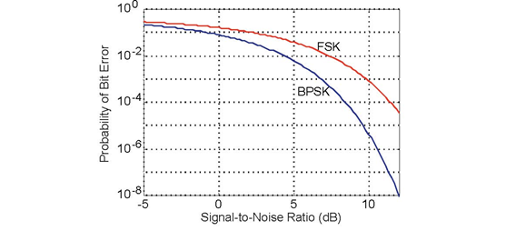
The probability that the matched-filter receiver makes an error on any bit transmission is plotted against the signal-to-noise ratio of the received signal. The upper curve shows the performance of the FSK signal set, the lower (and therefore better) one the BPSK signal set.
Exercise 6.17.1
Derive the probability of error expression for the modulated BPSK signal set, and show that its performance identically equals that of the baseband BPSK signal set.
- 4899 reads
