


Are sales higher in those geographic areas where more is spent on advertising? Does spending more on preventive maintenance reduce down-time? Are production workers with more seniority assigned the most popular jobs? All of these questions ask how the two variables move up and down together; when one goes up, does the other also rise? when one goes up does the other go down? Does the level of one have no effect on the level of the other? Statisticians measure the way two variables move together by measuring the correlation coefficient between the two.
Correlation will be discussed again in the next chapter, but it will not hurt to hear about the idea behind it twice. The basic idea is to measure how well two variables are tied together. Simply looking at the word, you can see that it means co-related. If whenever variable X goes up by 1, variable Y changes by a set amount, then X and Y are perfectly tied together, and a statistician would say that they are perfectly correlated. Measuring correlation usually requires interval data from normal populations, but a procedure to measure correlation from ranked data has been developed. Regular correlation coefficients range from -1 to +1. The sign tells you if the two variables move in the same direction (positive correlation) or in opposite directions (negative correlation) as they change together. The absolute value of the correlation coefficient tells you how closely tied together the variables are; a correlation coefficient close to +1 or to -1 means they are closely tied together, a correlation coefficient close to 0 means that they are not very closely tied together. The non-parametric Spearman's Rank Correlation Coefficient is scaled so that it follows these same conventions.
The true formula for computing the Spearman's Rank Correlation Coefficient is complex. Most people using rank correlation compute the coefficient with a computer program, but looking at the equation will help you see how Spearman's Rank Correlation works. It is:
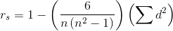
where:
n = the number of observations
d = the difference between the ranks for an observation
Keep in mind that we want this non-parametric correlation coefficient to range from -1 to +1 so that it acts like the parametric correlation coefficient. Now look at the equation. For a given
sample size, n, the only thing that will vary is  . If the
samples are perfectly positively correlated, then the same observation will be ranked first for both variables, another observation ranked second for both variables, etc. That means that each
difference in ranks, d, will be zero, the numerator of the fraction at the end of the equation will be zero, and that fraction will be zero. Subtracting zero from one leaves one, so if the
observations are ranked in the same order by both variables, the Spearman's Rank Correlation Coefficient is +1. Similarly, if the observations are ranked in exactly the opposite order by the
two variables, there will many large d2's, and
. If the
samples are perfectly positively correlated, then the same observation will be ranked first for both variables, another observation ranked second for both variables, etc. That means that each
difference in ranks, d, will be zero, the numerator of the fraction at the end of the equation will be zero, and that fraction will be zero. Subtracting zero from one leaves one, so if the
observations are ranked in the same order by both variables, the Spearman's Rank Correlation Coefficient is +1. Similarly, if the observations are ranked in exactly the opposite order by the
two variables, there will many large d2's, and  will be at its maximum. The rank correlation coefficient should equal -1, so you want to subtract 2 from 1 in the equation. The middle part of the equation, 6/n(n2-1), simply scales
 so that the whole term equals 2. As n grows larger,
  will grow larger if the two variables produce exactly opposite
rankings. At the same time, n(n2-1) will grow larger so that 6/n(n2-1) will grow smaller.
will grow larger if the two variables produce exactly opposite
rankings. At the same time, n(n2-1) will grow larger so that 6/n(n2-1) will grow smaller.
Colonial Milling Company produces flour, corn meal, grits, and muffin, cake, and quickbread mixes. They are considering introducing a new product, Instant Cheese Grits mix. Cheese grits is a dish made by cooking grits, combining the cooked grits with cheese and eggs, and then baking the mixture. It is a southern favorite in the United States, but because it takes a long time to cook, is not served much anymore. The Colonial mix will allow someone to prepare cheese grits in 20 minutes in only one pan, so if it tastes right, it should be a good-selling product in the South. Sandy Owens is the product manager for Instant Cheese Grits, and is deciding what kind of cheese flavoring to use. Nine different cheese flavorings have been successfully tested in production, and samples made with each of those nine flavorings have been rated by two groups: first, a group of food experts, and second, a group of potential customers. The group of experts was given a taste of three dishes of "homemade" cheese grits and ranked the samples according to how well they matched the real thing. The customers were given the samples and asked to rank them according to how much they tasted like "real cheese grits should taste". Over time, Colonial has found that using experts is a better way of identifying the flavorings that will make a successful product, but they always check the experts' opinion against a panel of customers. Sandy must decide if the experts and customers basically agree. If they do, then she will use the flavoring rated first by the experts. The data from the taste tests is in Table 7.6 Data from two taste tests of cheese flavorings.
|
Expert ranking |
Consumer ranking |
|
|
Flavoring |
||
|
NYS21 |
7 |
8 |
|
K73 |
4 |
3 |
|
K88 |
1 |
4 |
|
Ba4 |
8 |
6 |
|
Bc11 |
2 |
5 |
|
McA A |
3 |
1 |
|
McA A |
9 |
9 |
|
WIS4 |
5 |
2 |
|
WIS43 |
6 |
7 |
Sandy decides to use the SAS statistical software that Colonial has purchased. Her hypotheses are:
H0: The correlation between the expert and consumer rankings is zero or negative.
Ha: The correlation is positive.
Sandy will decide that the expert panel does know best if the data supports Ha : that there is a positive correlation between the experts and the consumers. She goes to a table that shows what value of the Spearman's Rank Correlation Coefficient will separate one tail from the rest of the sampling distribution if there is no association in the population. A portion of such a table is in Table 7.7 Some one-tail critical values for Spearman's Rank Correlation Coefficient.
| n | a=0.5 | a=0.25 | a=.10 |
| 5 | 0.9 | ||
| 6 | 0.829 | 0.886 | 0.943 |
| 7 | 0.714 | 0.786 | 0.893 |
| 8 | 0.643 | 0.738 | 0.833 |
| 9 | 0.6 | 0.683 | 0.783 |
| 10 | 0.564 | 0.648 | 0.745 |
| 11 | 0.523 | 0.623 | 0.736 |
| 12 | 0.497 | 0.591 | 0.703 |
Using  , going across the n = 9 row in Table 7.7, Sandy sees that if H0 : is true, only .05 of all samples will have an rs
greater than .600. Sandy decides that if her sample rank correlation is greater than .600, the data supports the alternative, and flavoring K88, the one ranked highest by the experts, will be
used. She first goes basck to the two sets of rankings and finds the difference in the rank given each flavor by the two groups, squares those differences and adds them together:
, going across the n = 9 row in Table 7.7, Sandy sees that if H0 : is true, only .05 of all samples will have an rs
greater than .600. Sandy decides that if her sample rank correlation is greater than .600, the data supports the alternative, and flavoring K88, the one ranked highest by the experts, will be
used. She first goes basck to the two sets of rankings and finds the difference in the rank given each flavor by the two groups, squares those differences and adds them together:
| Expert ranking | Consumer ranking | difference | d² | |
| Flavoring | ||||
| NYS21 | 7 | 8 | -1 | 1 |
| K73 | 4 | 3 | 1 | 1 |
| K88 | 1 | 4 | -3 | 9 |
| Ba4 | 8 | 6 | 2 | 4 |
| Bc11 | 2 | 5 | -3 | 9 |
| McA A | 3 | 1 | 2 | 4 |
| McA A | 9 | 9 | 0 | 0 |
| WIS 4 | 5 | 2 | 3 | 9 |
| WIS 43 | 6 | 7 | -1 | 1 |
|
sum = 38
|
||||
Then she uses the formula from above to find her Spearman rank correlation coefficient:
1-[6/(9)(92-1)][38] = 1 -.3166 = .6834
Her sample correlation coefficient is .6834, greater than .600, so she decides that the experts are reliable, and decides to use flavoring K88. Even though Sandy has ordinal data that only ranks the flavorings, she can still perform a valid statistical test to see if the experts are reliable. Statistics has helped another manager make a decision.
- 2000 reads
