The t-distribution

Available under Creative Commons-ShareAlike 4.0 International License.

The central limit theorem tells us about the relationship between the sampling distribution of means and the original population. Notice that if we want to know the variance of the sampling distribution we need to know the variance of the original population. You do not need to know the variance of the sampling distribution to make a point estimate of the mean, but other, more elaborate, estimation techniques require that you either know or estimate the variance of the population. If you reflect for a moment, you will realize that it would be strange to know the variance of the population when you do not know the mean. Since you need to know the population mean to calculate the population variance and standard deviation, the only time when you would know the population variance without the population mean are examples and problems in textbooks. The usual case occurs when you have to estimate both the population variance and mean. Statisticians have figured out how to handle these cases by using the sample variance as an estimate of the population variance (and being able to use that to estimate the variance of the sampling distribution). Remember that s² is an unbiased estimator of . Remember, too, that the variance of the sampling distribution of means is related to the variance of the original population according to the equation:

so, the estimated standard deviation of a sampling distribution of means is:

Following this thought, statisticians found that if they took samples of a constant size from a normal population, computed a statistic called a "t-score" for each sample, and put those into a relative frequency distribution, the distribution would be the same for samples of the same size drawn from any normal population. The shape of this sampling distribution of t's varies somewhat as sample size varies, but for any n it's always the same. For example, for samples of 5, 90% of the samples have t-scores between -1.943 and +1.943, while for samples of 15, 90% have t-scores between ± 1.761. The bigger the samples, the narrower the range of scores that covers any particular proportion of the samples. That t-score is computed by the formula:

By comparing the formula for the t-score with the formula for the z-score, you will be able to see that the t is just an estimated z. Since there is one t-score for each sample, the t is just another sampling distribution. It turns out that there are other things that can be computed from a sample that have the same distribution as this t. Notice that we've used the sample standard deviation, s, in computing each t-score. Since we've used s, we've used up one degree of freedom. Because there are other useful sampling distributions that have this same shape, but use up various numbers of degrees of freedom, it is the usual practice to refer to the t-distribution not as the distribution for a particular sample size, but as the distribution for a particular number of degrees of freedom. There are published tables showing the shapes of the t-distributions, and they are arranged by degrees of freedom so that they can be used in all situations.

Looking at the formula, you can see that the mean t-score will be zero since the mean equals . Each t-distribution is symmetric, with half of the t-scores being positive and half negative because we know from the central limit theorem that the sampling distribution of means is normal, and therefore symmetric, when the original population is normal.

An excerpt from a typical t-table is printed below. Note that there is one line each for various degrees of freedom. Across the top are the proportions of the distributions that will be left out in the tail--the amount shaded in the picture. The body of the table shows which t-score divides the bulk of the distribution of t's for that df from the area shaded in the tail, which t-score leaves that proportion of t's to its right. For example, if you chose all of the possible samples with 9 df, and found the t-score for each, .025 (2 1/2 %) of those samples would have t-scores greater than 2.262, and .975 would have t-scores less than 2.262.

Figure 2.1 A sampling of a student's t-table. 

The table shows the probability of exceeding the value in the body. With 5 df, there is a .05 probability that a sample will have a t-score > 2.015. 

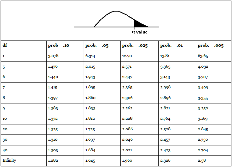
Since the t-distributions are symmetric, if 2 1/2% (.025) of the t's with 9 df are greater than 2.262, then 2 1/2% are less than -2.262. The middle 95% (.95) of the t's, when there are 9 df, are between -2.262 and +2.262. The middle .90 of t=scores when there are 14 df are between ±1.761, because -1.761 leaves .05 in the left tail and +1.761 leaves .05 in the right tail. The t-distribution gets closer and closer to the normal distribution as the number of degrees of freedom rises. As a result, the last line in the t-table, for infinity df, can also be used to find the z-scores that leave different proportions of the sample in the tail.

What could Kevin have done if he had been asked "about how much does a pair of size 11 socks weigh?" and he could not easily find good data on the population? Since he knows statistics, he could take a sample and make an inference about the population mean. Because the distribution of weights of socks is the result of a manufacturing process, it is almost certainly normal. The characteristics of almost every manufactured product are normally distributed. In a manufacturing process, even one that is precise and well-controlled, each individual piece varies slightly as the temperature varies some, the strength of the power varies as other machines are turned on and off, the consistency of the raw material varies slightly, and dozens of other forces that affect the final outcome vary slightly. Most of the socks, or bolts, or whatever is being manufactured, will be very close to the mean weight, or size, with just as many a little heavier or larger as there are that are a little lighter or smaller. Even though the process is supposed to be producing a population of "identical" items, there will be some variation among them. This is what causes so many populations to be normally distributed. Because the distribution of weights is normal, he can use the t-table to find the shape of the distribution of sample t-scores. Because he can use the t-table to tell him about the shape of the distribution of sample t-scores, he can make a good inference about the mean weight of a pair of socks. This is how he could make that inference:

STEP 1. Take a sample of n, say 15, pairs size 11 socks and carefully weigh each pair.
STEP 2. Find and s for his sample.
STEP 3 (where the tricky part starts). Look at the t-table, and find the t-scores that leave some proportion, say .95, of sample t's with n-1 df in the middle.
STEP 4 (the heart of the tricky part). Assume that his sample has a t-score that is in the middle part of the distribution of t-scores.
STEP 5 (the arithmetic). Take his , s, n, and t's from the t-table, and set up two equations, one for each of his two table t-values. When he solves each of these equations for m, he will find an interval that he is 95% sure (a statistician would say "with .95 confidence") contains the population mean.

Kevin decides this is the way he will go to answer the question. His sample contains pairs of socks with weights of :
4.36, 4.32, 4.29, 4.41, 4.45, 4.50, 4.36, 4.35, 4.33, 4.30, 4.39, 4.41, 4.43, 4.28, 4.46 oz.

He finds his sample mean, ounces, and his sample standard deviation (remembering to use the sample formula), s = .067 ounces. The t-table tells him that .95 of sample t's with 14 df are between ±2.145. He solves these two equations for :

and

finding ounces and ounces. With these results, Kevin can report that he is "95 per cent sure that the mean weight of a pair of size 11 socks is between 4.366 and 4.386 ounces". Notice that this is different from when he knew more about the population in the previous example.