


Another common interval estimation task is to estimate the variance of a population. High quality products not only need to have the proper mean dimension, the variance should be small. The estimation of population variance follows the same strategy as the other estimations. By choosing a sample and assuming that it is from the middle of the population, you can use a known sampling distribution to find a range of values that you are confident contains the population variance. Once again, we will use a sampling distribution that statisticians have discovered forms a link between samples and populations.
Take a sample of size n from a normal population with known variance, and compute a statistic called "  " (pronounced "chi square") for that sample using the following formula:
You can see that  will always be positive, because both the
numerator and denominator will always be positive. Thinking it through a little, you can also see that as n gets larger,
will always be positive, because both the
numerator and denominator will always be positive. Thinking it through a little, you can also see that as n gets larger,  ,will generally be larger since the numerator will tend to be larger as more and more
  are summed together. It should not be too surprising by now to find out that if all of
the possible samples of a size n are taken from any normal population, that when
are summed together. It should not be too surprising by now to find out that if all of
the possible samples of a size n are taken from any normal population, that when  is computed for each sample and those
  are arranged into a relative frequency distribution, the distribution is always the same.
Because the size of the sample obviously affects  , there is a
different distribution for each different sample size. There are other sample statistics that are distributed like
, there is a
different distribution for each different sample size. There are other sample statistics that are distributed like  , so, like the t-distribution, tables of the
  distribution are arranged by degrees of freedom so that they can be used in any procedure where appropriate. As you might expect,
in this procedure, df = n-1. A portion of a
distribution are arranged by degrees of freedom so that they can be used in any procedure where appropriate. As you might expect,
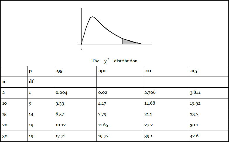
in this procedure, df = n-1. A portion of a  table is
reproduced below.
table is
reproduced below.
Variance is important in quality control because you want your product to be consistently the same. John McGrath has just returned from a seminar called "Quality Socks, Quality Profits". He learned something about variance, and has asked Kevin to measure the variance of the weight of Foothill's socks. Kevin decides that he can fulfill this request by using the data he collected when Mr. McGrath asked about the average weight of size 11 men's dress socks. Kevin knows that the sample variance is an unbiased estimator of the population variance, but he decides to produce an interval estimate of the variance of the weight of pairs of size 11 men's socks. He also decides that .90 confidence will be good until he finds out more about what Mr. McGrath wants.
Kevin goes and finds the data for the size 11 socks, and gets ready to use the  distribution to make a .90 confidence interval estimate of the variance of the weights of socks. His sample has 15 pairs in it,
so he will have 14 df. From the
distribution to make a .90 confidence interval estimate of the variance of the weights of socks. His sample has 15 pairs in it,
so he will have 14 df. From the  table he sees that .95 of
 are greater than 6.57 and only .05 are greater than 23.7 when
there are 14 df. This means that .90 are between 6.57 and 23.7. Assuming that his sample has a
are greater than 6.57 and only .05 are greater than 23.7 when
there are 14 df. This means that .90 are between 6.57 and 23.7. Assuming that his sample has a  that is in the middle .90, Kevin gets ready to compute the limits of his interval. He notices that he will have to find
  and decides to use his spreadsheet program rather than find
 fifteen times. He puts the original sample values in
the first column, and has the program compute the mean. Then he has the program find
fifteen times. He puts the original sample values in
the first column, and has the program compute the mean. Then he has the program find  fifteen times. Finally, he has the spreadsheet sum up the squared differences and finds 0.062.
Kevin then takes the  formula, and solves it twice, once by
setting
formula, and solves it twice, once by
setting  equal to 6.57:
Solving for  , he finds one limit for his interval is .0094.
He solves the second time by setting
, he finds one limit for his interval is .0094.
He solves the second time by setting  :
:
and find that the other limit is .0026. Armed with his data, Kevin reports to Mr. McGrath that "with .90 confidence, the variance of weights of size 11 men's socks is between .0026 and .0094."
- 5368 reads
