Testing your regression. Does this equation really help predict?

Available under Creative Commons-ShareAlike 4.0 International License.

Returning to the laundry soap illustration, the easiest way to predict how much laundry soap a particular family (or any family, for that matter) uses would be to take a sample of families, find the mean soap use of that sample, and use that sample mean for your prediction, no matter what the family size. To test to see if the regression equation really helps, see how much of the error that would be made using the mean of all of the y's to predict is eliminated by using the regression equation to predict. By testing to see if the regression helps predict, you are testing to see if there is a functional relationship in the population.

Imagine that you have found the mean soap use for the families in a sample, and for each family you have made the simple prediction that soap use will be equal to the sample mean, $\bar{y}$ . This is not a very sophisticated prediction technique, but remember that the sample mean is an unbiased estimator of population mean, so "on average" you will be right. For each family, you could compute your "error" by finding the difference between your prediction (the sample mean, $\bar{y}$ ) and the actual amount of soap used.

As an alternative way to predict soap use, you can have a computer find the intercept, $\alpha$ , and slope, $\beta$ , of the sample regression line. Now, you can make another prediction of how much soap each family in the sample uses by computing:

$\hat{y}=\alpha +\beta \left ( familysize \right )$

Once again, you can find the error made for each family by finding the difference between soap use predicted using the regression equation, ŷ, and actual soap use, $\bar{y}$ . Finally, find how much using the regression improves your prediction by finding the difference between soap use predicted using the mean, $\bar{y}$ , and soap use predicted using regression, ŷ. Notice that the measures of these differences could be positive or negative numbers, but that "error" or "improvement" implies a positive distance. There are probably a few families where the error from using the regression is greater than the error from using the mean, but generally the error using regression will be smaller.

If you use the sample mean to predict the amount of soap each family uses, your error is $(y-\bar{y})$ for each family. Squaring each error so that worries about signs are overcome, and then adding the squared errors together, gives you a measure of the total mistake you make if you use to predict y. Your total mistake is $\sum \left ( y-\bar{y} \right )^{2}$ The total mistake you make using the regression model would be $\sum \left ( y-\hat{y} \right )^{2}$ . The difference between the mistakes, a raw measure of how much your prediction has improved, is $\sum \left ( \hat{y}-\bar{y} \right )^{2}$ . To make this raw measure of the improvement meaningful, you need to compare it to one of the two measures of the total mistake. This means that there are two measures of "how good" your regression equation is. One compares the improvement to the mistakes still made with regression. The other compares the improvement to the mistakes that would be made if the mean was used to predict. The first is called an F-score because the sampling distribution of these measures follows the F-distribution seen in the “F-test and one-way anova” chapter. The second is called R² , or the "coefficient of determination".

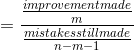
All of these mistakes and improvements have names, and talking about them will be easier once you know those names. The total mistake made using the sample mean to predict, $\sum \left ( y-\bar{y} \right )^{2}$ , is called the "sum of squares, total". The total mistake made using the regression, $\sum \left ( y-\hat{y} \right )^{2}$ , is called the "sum of squares, residual" or the "sum of squares, error". The total improvement made by using regression, $\sum \left ( \hat{y}-\bar{y} \right )^{2}$ is called the "sum of squares, regression" or "sum of squares, model". You should be able to see that:

Sum of Squares Total = Sum of Squares Regression + Sum of Squares Residual

$\sum\left ( y-\bar{y} \right ) ^{2}=\sum \left ( \hat{y}-\bar{y} \right )^{2}+\sum \left ( y-\hat{y} \right )^{2}$

The F-score is the measure usually used in a hypothesis test to see if the regression made a significant improvement over using the mean. It is used because the sampling distribution of F-scores that it follows is printed in the tables at the back of most statistics books, so that it can be used for hypothesis testing. There is also a good set of F-tables at http://www.itl.nist.gov/div898/handbook/eda/section3/eda3673.htm. It works no matter how many explanatory variables are used. More formally if there was a population of multivariate observations, ( y ,x₁ ,x₂ , ..., x_m) , and there was no linear relationship between y and the x's, so that $y\neq f(x_{1},x_{2},...,x_{m})$ , if samples of n observations are taken, a regression equation estimated for each sample, and a statistic, F, found for each sample regression, then those F's will be distributed like those in the F-table with (m, n-m-1) df. That F is:

$F= \frac{\frac{\sum of Squares Regression}{m}}{\frac{\sum of Squares Residual}{\left ( n-m-1 \right )}}$

$=\frac{\frac{improvement made}{m}}{\frac{mistakes still made}{n-m-1}}$

$F=\frac{\frac{\sum \left ( \hat{y}-\bar{y} \right )^{2}}{m}}{\frac{\sum \left ( y-\hat{y} \right )^{2}}{\left ( n-m-1 \right )}}$

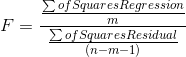
where: n is the size of the sample
m is the number of explanatory variables (how many x's there are in the regression equation).

If, $\sum \left ( \hat{y}-\bar{y} \right )^{2}$ the sum of squares regression (the improvement), is large relative to $\sum \left ( y-\hat{y} \right )^{2}$ , the sum of squares residual (the mistakes still made), then the F-score will be large. In a population where there is no functional relationship between y and the x's, the regression line will have a slope of zero (it will be flat), and the $\hat{y}$ will be close to y. As a result very few samples from such populations will have a large sum of squares regression and large F-scores. Because this F-score is distributed like the one in the F-tables, the tables can tell you whether the F-score a sample regression equation produces is large enough to be judged unlikely to occur if $y\neq f(x_{1},x_{2},...,x_{m})$ . The sum of squares regression is divided by the number of explanatory variables to account for the fact that it always decreases when more variables are added. You can also look at this as finding the improvement per explanatory variable. The sum of squares residual is divided by a number very close to the number of observations because it always increases if more observations are added. You can also look at this as the approximate mistake per observation.

$H_{0}:y\neq f(x_{1},x_{2},...,x_{m})$

To test to see if a regression equation was worth estimating, test to see if there seems to be a functional relationship:

$H_{a}:y=f(x_{1},x_{2},...,x_{m})$

This might look like a two-tailed test since H₀ : has an equal sign. But, by looking at the equation for the F-score you should be able to see that the data supports H_a : only if the F-score is large. This is because the data supports the existence of a functional relationship if sum of squares regression is large relative to the sum of squares residual. Since F-tables are usually one-tailed tables, choose an α, go to the F-tables for that α and (m, n-m1) df, and find the table F. If the computed F is greater than the table F, then the computed F is unlikely to have occurred if H₀ : is true, and you can safely decide that the data supports H_a :. There is a functional relationship in the population.

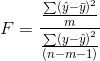
The other measure of how good your model is, the ratio of the improvement made using the regression to the mistakes made using the mean is called "R-square", usually written R². While R² is not used to test hypotheses, it has a more intuitive meaning than the F-score. R² is found by:

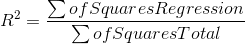
$R^{2}=\frac{\sum of Squares Regression}{\sum of Squares Total}$

The numerator is the improvement regression makes over using the mean to predict, the denominator is the mistakes made using the mean, so R² simply shows what proportion of the mistakes made using the mean are eliminated by using regression.

Cap Gains, who in the example earlier in this chapter, was trying to see if there is a relationship between price-earnings ratio (P/E) and a "time to buy" rating (TtB), has decided to see if he can do a good job of predicting P/E by using a regression of TtB and profits as a percent of net worth (per cent profit) on P/E. He collects a sample of (P/E, TtB, per cent profit) for 25 firms, and using a computer, estimates the function

$P/E=\alpha +\beta _{1}TtB+\beta _{2}profit$

He again uses the SAS program, and his computer printout gives him the results in Figure 8.2 Cap's SAS computer printout. This time he notices that there are two pages in the printout.

Figure 8.2 Cap's SAS computer printout

The equation the regression estimates is:
P/E=27.281-3.772TtB-0.012Profit

Cap can now test three hypotheses. First, he can use the F-score to test to see if the regression model improves his ability to predict P/E. Second and third, he can use the t-scores to test to see if the slopes of TtB and Profit are different from zero.

To conduct the first test, Cap decides to choose an α = .10. The F-score is the regression or model mean square over the residual or error mean square, so the df for the F-statistic are first the df for the model and second the df for the error. There are 2,23 df for the F-test. According to his F-table, with 2.23 degrees of freedom, the critical F-score for $\alpha=.10$ is 2.55. His hypotheses are:

$H_{0}:P/E\neq f(TtB,Profit)$

$H_{a}:P/E= f(TtB,Profit)$

Because the F-score from the regression, 2.724, is greater than the critical F-score, 2.55, Cap decides that the data supports H_a : and concludes that the model helps him predict P/E. There is a functional relationship in the a population.

Cap can also test to see if P/E depends on TtB and Profit individually by using the t-scores for the parameter estimates. There are (n-m-1)=23 degrees of freedom. There are two sets of hypotheses, one set for $\beta _{1}$ , the slope for TtB, and one set for $\beta _{2}$ , the slope for Profit. He expects that $\beta _{1}$ , the slope for TtB, will be negative, but he does not have any reason to expect that $\beta _{2}$ will be either negative or positive. Therefore, Cap will use a one-tail test on $\beta _{1}$ , and a two-tail test on $\beta _{2}$ :

$H_{0}:\beta _{1}\geq 0$ $H_{0}:\beta _{2}= 0$
$H_{a}:\beta _{1}< 0$ $H_{a}:\beta _{2}= 0$

Since he has one one-tail test and one two-tail test, the t-values he chooses from the t-table will be different for the two tests. Using $\alpha=.10$ , Cap finds that his t-score for $\beta_{1}$ the one-tail test, will have to be more negative than -1.32 before the data supports P/E being negatively dependent on TtB. He also finds that his t-score for $\beta _{2}$ , the two-tail test, will have to be outside ±1.71 to decide that P/E depends upon Profit. Looking back at his printout and checking the t-scores, Cap decides that Profit does not affect P/E, but that higher TtB ratings mean a lower P/E. Notice that the printout also gives a t-score for the intercept, so Cap could test to see if the intercept equals zero or not.

Though it is possible to do all of the computations with just a calculator, it is much easier, and more dependably accurate, to use a computer to find regression results. Many software packages are available, and most spreadsheet programs will find regression slopes. I left out the steps needed to calculate regression results without a computer on purpose, for you will never compute a regression without a computer (or a high end calculator) in all of your working years, and there is little most people can learn about how regression works from looking at the calculation method.

927 reads

You are here

Testing your regression. Does this equation really help predict?