Testing your regression: does y really depend upon x?

Available under Creative Commons-ShareAlike 4.0 International License.

Understanding that there is a distribution of y (soap use) values at each x (family size) is the key for understanding how regression results from a sample can be used to test the hypothesis that there is (or is not) a relationship between x and y. When you hypothesize that y = f(x), you hypothesize that the slope of the line ( $\beta$ in $y=\alpha+\beta x+\epsilon$ ) is not equal to zero. If $\beta$ was equal to zero, changes in x would not cause any change in y. Choosing a sample of families, and finding each family's size and soap use, gives you a sample of (x, y). Finding the equation of the line that best fits the sample will give you a sample intercept, a, and a sample slope, b. These sample statistics are unbiased estimators of the population intercept, $\alpha$ , and slope, $\beta$ . If another sample of the same size is taken another sample equation could be generated. If many samples are taken, a sampling distribution of sample $\beta$ 's, the slopes of the sample lines, will be generated. Statisticians know that this sampling distribution of b's will be normal with a mean equal to $\beta$ , the population slope. Because the standard deviation of this sampling distribution is seldom known, statisticians developed a method to estimate it from a single sample. With this estimated s_b , a t-statistic for each sample can be computed:

$t=\frac{b-\beta }{estimated \sigma _{b} }=\frac{b-\beta }{s_{b}}$

where n = sample size
           m = number of explanatory (x) variables
          b = sample slope
          $\beta$ = population slope
         s_b = estimated standard deviation of b's, often called the "standard error".

These t's follow the t-distribution in the tables with n-m-1 df.

Computing s_b is tedious, and is almost always left to a computer, especially when there is more than one explanatory variable. The estimate is based on how much the sample points vary from the regression line. If the points in the sample are not very close to the sample regression line, it seems reasonable that the population points are also widely scattered around the population regression line and different samples could easily produce lines with quite varied slopes. Though there are other factors involved, in general when the points in the sample are farther from the regression line s_b is greater. Rather than learn how to compute s_b , it is more useful for you to learn how to find it on the regression results that you get from statistical software. It is often called the "standard error" and there is one for each independent variable. The printout in Table 8.1 Typical statistical package output for regression is typical.

Table 8.1 Typical statistical package output for regression
Variable	DF	Parameter	Std Error	t-score
Intercept	1	27.01	4.07	6.64
TtB	1	-3.75	1.54	-2.43

You will need these standard errors in order to test to see if y depends upon x or not. You want to test to see if the slope of the line in the population, $\beta$ , is equal to zero or not. If the slope equals zero, then changes in x do not result in any change in y. Formally, for each independent variable, you will have a test of the hypotheses:

$H_{0}:\beta =0$

$H_{a}:\beta \neq 0$

if the t-score is large (either negative or positive), then the sample b is far from zero (the hypothesized $\beta$ ), and H_a : should be accepted. Substitute zero for b into the t-score equation, and if the t-score is small, b is close a enough to zero to accept H₀ :. To find out what t-value separates "close to zero" from "far from zero", choose an $\alpha$ , find the degrees of freedom, and use a t-table to find the critical value of t. Remember to halve $\alpha$ when conducting a two-tail test like this. The degrees of freedom equal n - m - 1, where n is the size of the sample and m is the number of independent x variables. There is a separate hypothesis test for each independent variable. This means you test to see if y is a function of each x separately. You can also test to see if $\beta> 0$ (or $\beta< 0$ ) rather than simply if $\beta\neq 0$ by using a one-tail test, or test to see if his some particular value by substituting that value for β when computing the sample t-score.

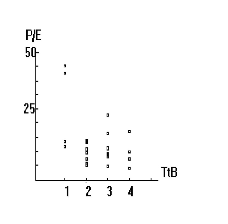
Casper Gains has noticed that various stock market newsletters and services often recommend stocks by rating if this is a good time to buy that stock. Cap is cynical and thinks that by the time a newsletter is published with such a recommendation the smart investors will already have bought the stocks that are timely buys, driving the price up. To test to see if he is right or not, Cap collects a sample of the price-earnings ratio (P/E) and the "time to buy" rating (TtB) for 27 stocks. P/E measures the value of a stock relative to the profitability of the firm. Many investors search for stocks with P/E's that are lower than would be expected, so a high P/E probably means that the smart investors have discovered the stock. He decides to estimate the functional relationship between P/E and TtB using regression. Since a TtB of 1 means "excellent time to buy", and a TtB of 4 means "terrible time to buy", Cap expects that the slope, $\beta$ , of the line $P/E=\alpha+\beta*TtB+\epsilon$ will be negative. Plotting out the data gives the graph in Figure 8.1 A plot of Cap's stock data.

Figure 8.1 A plot of Cap's stock data

Entering the data into the computer, and using the SAS statistical software Cap has at work to estimate the function, yields the output given above.

Because Cap Gains wants to test to see if P/E is already high by the time a low TtB rating is published, he wants to test to see if the slope of the line, which is estimated by the parameter for TtB, is negative or not. His hypotheses are:

$H_{0}:\beta \geq 0$

$H_{a}:\beta < 0$

He should use a one-tail t-test, because the alternative is "less than zero", not simply "not equal to zero". Using an $\alpha=.05$ , and noting that there are n-m-1, 26-1-1 = 24 degrees of freedom, Cap goes to the t-table and finds that he will accept H_a : if the t-score for the slope of the line with respect to TtB is smaller (more negative) than -1.711. Since the t-score from the computer output is -2.43, Cap should accept H_a : and conclude that by the time the TtB rating is published, the stock price has already been bid up, raising P/E. Buying stocks only on the basis of TtB is not an easy way to make money quickly in the stock market. Cap's cynicism seems to be well founded.

Both the laundry soap and Cap Gains's examples have an independent variable that is always a whole number. Usually, all of the variables are continuous, and to use the hypothesis test developed in this chapter all of the variables really should be continuous. The limit on the values of x in these examples is to make it easier for you to understand how regression works; these are not limits on using regression.

1364 reads

You are here

Testing your regression: does y really depend upon x?