


The supply curve for an industry, such as coffee, includes all the sellers in the industry. A change in the number of sellers in an industry changes the quantity available at each price and thus changes supply. An increase in the number of sellers supplying a good or service shifts the supply curve to the right; a reduction in the number of sellers shifts the supply curve to the left.
The market for cellular phone service has been affected by an increase in the number of firms offering the service. Over the past decade, new cellular phone companies emerged, shifting the supply curve for cellular phone service to the right.
Heads Up!
There are two special things to note about supply curves. The first is similar to the Heads Up! on demand curves: it is important to distinguish carefully between changes in supply and changes in quantity supplied. A change in supply results from a change in a supply shifter and implies a shift of the supply curve to the right or left. A change in price produces a change in quantity supplied and induces a movement along the supply curve. A change in price does not shift the supply curve.
The second caution relates to the interpretation of increases and decreases in supply. Notice that in Figure 3.2 an increase in supply is shown as a shift of the supply curve to the right; the curve shifts in the direction of increasing quantity with respect to the horizontal axis. In Figure 3.3 a reduction in supply is shown as a shift of the supply curve to the left; the curve shifts in the direction of decreasing quantity with respect to the horizontal axis. Because the supply curve is upward sloping, a shift to the right produces a new curve that in a sense lies “below” the original curve. Students sometimes make the mistake of thinking of such a shift as a shift “down” and therefore as a reduction in supply. Similarly, it is easy to make the mistake of showing an increase in supply with a new curve that lies “above” the original curve. But that is a reduction in supply! To avoid such errors, focus on the fact that an increase in supply is an increase in the quantity supplied at each price and shifts the supply curve in the direction of increased quantity on the horizontal axis. Similarly, a reduction in supply is a reduction in the quantity supplied at each price and shifts the supply curve in the direction of a lower quantity on the horizontal axis.

KEY TAKEAWAYS
- The quantity supplied of a good or service is the quantity sellers are willing to sell at a particular price during a particular period, all other things unchanged.
- A supply schedule shows the quantities supplied at different prices during a particular period, all other things unchanged.
- A supply curve shows this same information graphically.
- A change in the price of a good or service causes a change in the quantity supplied—a movement along the supply curve.
- A change in a supply shifter causes a change in supply, which is shown as a shift of the supply curve. Supply shifters include prices of factors of production, returns from alternative activities, technology, seller expectations, natural events, and the number of sellers.
- An increase in supply is shown as a shift to the right of a supply curve; a decrease in supply is shown as a shift to the left.
TRY IT!
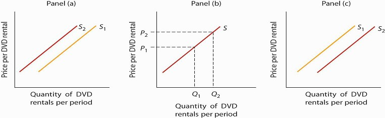
If all other things are unchanged, what happens to the supply curve for DVD rentals if there is (a) an increase in wages paid to DVD rental store clerks, (b) an increase in the price of DVD rentals, or (c) an increase in the number of DVD rental stores? Draw a graph that shows what happens to the supply curve in each circumstance. The supply curve can shift to the left or to the right, or stay where it is. Remember to label the axes and curves, and remember to specify the time period (e.g., “DVDs rented per week”).
Case in Point: The Monks of St. Benedict's Get Out of the Egg Business
It was cookies that lured the monks of St. Benedict’s out of the egg business, and now private retreat sponsorship is luring them away from cookies.
St. Benedict’s is a Benedictine monastery, nestled on a ranch high in the Colorado Rockies, about 20 miles down the road from Aspen. The monastery’s 15 monks operate the ranch to support
themselves and to provide help for poor people in the area. They lease out about 3,500 acres of their land to cattle and sheep grazers, produce cookies, and sponsor private retreats. They
used to produce eggs.
Attracted by potential profits and the peaceful nature of the work, the monks went into the egg business in 1967. They had 10,000 chickens producing their Monastery Eggs brand. For a while,
business was good. Very good. Then, in the late 1970s, the price of chicken feed started to rise rapidly. “When we started in the business, we were paying $60 to $80 a ton for
feed—delivered,” recalls the monastery’s abbot, Father Joseph Boyle. “By the late 1970s, our cost had more than doubled. We were paying $160 to $200 a ton. That really hurt, because feed
represents a large part of the cost of producing eggs.” The monks adjusted to the blow.
“When grain prices were lower, we’d pull a hen off for a few weeks to molt, then return her to laying. After grain prices went up, it was 12 months of laying and into the soup pot,” Father
Joseph says. Grain prices continued to rise in the 1980s and increased the costs of production for all egg producers. It caused the supply of eggs to fall. Demand fell at the same time, as
Americans worried about the cholesterol in eggs. Times got tougher in the egg business. “We were still making money in the financial sense,” Father Joseph says. “But we tried an experiment in
1985 producing cookies, and it was a success. We finally decided that devoting our time and energy to the cookies would pay off better than the egg business, so we quit the egg business in
1986.” The mail-order cookie business was good to the monks. They sold 200,000 ounces of Monastery Cookies in 1987. By 1998, however, they had limited their production of cookies, selling
only locally and to gift shops. Since 2000, they have switched to “providing private retreats for individuals and groups—about 40 people per month,” according to Brother Charles.
The monks’ calculation of their opportunity costs revealed that they would earn a higher return through sponsorship of private retreats than in either cookies or eggs. This projection has
proved correct. And there is another advantage as well. “The chickens didn’t stop laying eggs on Sunday,” Father Joseph chuckles. “When we shifted to cookies we could take Sundays off. We
weren’t hemmed in the way we were with the chickens.” The move to providing retreats is even better in this regard. Since guests provide their own meals, most of the monastery’s effort goes
into planning and scheduling, which frees up even more of their time for other worldly as well as spiritual pursuits.
Source: Personal interviews.
ANSWER TO TRY IT! PROBLEM
DVD rental store clerks are a factor of production in the DVD rental market. An increase in their wages raises the cost of production, thereby causing the supply curve of DVD rentals to shift to the left [Panel (a)].
An increase in the price of DVD rentals does not shift the supply curve at all; rather, it corresponds to a movement upward to the right along the supply curve. At a higher price of P2 instead of P1, a greater quantity of DVD rentals, say Q2 instead of Q1, will be supplied [Panel (b)]. An increase in the number of stores renting DVDs will cause the supply curve to shift to the right [Panel (c)].
- 6011 reads
