


Summary
This chapter introduced a new tool: the concept of elasticity. Elasticity is a measure of the degree to which a dependent variable responds to a change in an independent variable. It is the percentage change in the dependent variable divided by the percentage change in the independent variable, all other things unchanged.
The most widely used elasticity measure is the price elasticity of demand, which reflects the responsiveness ofquantity demanded to changes in price. Demand is said to be price elastic if the absolute value of the price elasticity of demand is greater than 1, unit price elastic if it is equal to 1, and price inelastic if it is less than 1. The price elasticity of demand is useful in forecasting the response of quantity demanded to price changes; it is also useful for predicting the impact a price change will have on total revenue. Total revenue moves in the direction of the quantity change if demand is price elastic, it moves in the direction of the price change if demand is price inelastic, and it does not change if demand is unit price elastic. The most important determinants of the price elasticity of demand are the availability of substitutes, the importance of the item in household budgets, and time.
Two other elasticity measures commonly used in conjunction with demand are income elasticity and crossprice elasticity. The signs of these elasticity measures play important roles. A positive income elasticity tells us that a good is normal; a negative income elasticity tells us the good is inferior. A positive cross price elasticittells us that two goods are substitutes; a negative cross price elasticity tells us they are complements.
Elasticity of supply measures the responsiveness of quantity supplied to changes in price. The value of price elasticity of supply is generally positive. Supply is classified as being price elastic, unit price elastic, or price inelastic if price elasticity is greater than 1, equal to 1, or less than 1, respectively. The length of time over which supply is being considered is an important determinant of the price elasticity of supply.
CONCEPT PROBLEMS
- Explain why the price elasticity of demand is generally a negative number, except in the cases where thdemand curve is perfectly elastic or perfectly inelastic. What would be implied by a positive price elasticity of demand?
- Explain why the sign (positive or negative) of the cross price elasticity of demand is important.
- Explain why the sign (positive or negative) of the income elasticity of demand is important.
- Economists Dale Heien and Cathy Roheim Wessells found that the price elasticity of demand for fresh milk is −0.63 and the price elasticity of demand for cottage cheese is −1.1. Why do you think the elasticit estimates differ?
- The price elasticity of demand for health care has been estimated to be −0.2. Characterize this demand asprice elastic, unit price elastic, or price inelastic. The text argues that the greater the importance of an item in consumer budgets, the greater its elasticity. Health-care costs account for a relatively large share ohousehold budgets. How could the price elasticity of demand for health care be such a small number?
- Suppose you are able to organize an alliance that includes all farmers. They agree to follow the group’sinstructions with respect to the quantity of agricultural products they produce. What might the group seek to do? Why?
- Suppose you are the chief executive officer of a firm, and you have been planning to reduce your prices.Your marketing manager reports that the price elasticity of demand for your product is −0.65.
- How will this news affect your plans?
- Suppose the income elasticity of the demand for beans is −0.8. Interpret this number.
- Transportation economists generally agree that the cross price elasticity of demand for automobile usewith respect to the price of bus fares is about 0. Explain what this number means.
- Suppose the price elasticity of supply of tomatoes as measured on a given day in July is 0. Interpret this number.
- The price elasticity of supply for child-care workers was reported to be quite high, about 2. What will happen to the wages of child-care workers as demand for them increases, compared to what would happen if the measured price elasticity of supply were lower?
- The Case in Point on cigarette taxes and teen smoking suggests that a higher tax on cigarettes would reduce teen smoking and premature deaths. Should cigarette taxes therefore be raised?
NUMERICAL PROBLEMS
- Economist David Romer found that in introductory economics classes a 10% increase in class attendance is associated with a 4% increase in course grade. What is the elasticity of course
grade with respect to class attendance? Refer to Figure 5.2 and
- Using the arc elasticity of demand formula, compute the price elasticity of demand between points B and C.
- Using the arc elasticity of demand formula, compute the price elasticity of demand between points D and E.
- How do the values of price elasticity of demand compare? Why are they the same or different?
- Compute the slope of the demand curve between points B and C.
- Computer the slope of the demand curve between points D and E.
- How do the slopes compare? Why are they the same or different?
- Consider the following quote from The Wall Street Journal: “A bumper crop of oranges in Florida last year drove down orange prices. As juice marketers’ costs fell, they cut prices by as
much as 15%. That was enough to tempt some value-oriented customers: unit volume of frozen juices actually rose about 6% during the quarter.”
- Given these numbers, and assuming there were no changes in demand shifters for frozen orange juice, what was the price elasticity of demand for frozen orange juice?
- What do you think happened to total spending on frozen orange juice? Why?
- Suppose you are the manager of a restaurant that serves an average of 400 meals per day at an average price per meal of $20. On the basis of a survey, you have determined that reducing
the price of an average meal to $18 would increase the quantity demanded to 450 per day.
- Compute the price elasticity of demand between these two points.
- Would you expect total revenues to rise or fall? Explain.
- Suppose you have reduced the average price of a meal to $18 and are considering a further reduction to $16. Another survey shows that the quantity demanded of meals will increase from 450 to 500 per day. Compute the price elasticity of demand between these two points.
- Would you expect total revenue to rise or fall as a result of this second price reduction? Explain.
- Compute total revenue at the three meal prices. Do these totals confirm your answers in (b) and (d) above?
- The text notes that, for any linear demand curve, demand is price elastic in the upper half and price inelastic in the lower half. Consider the following demand curves:
- Compute the price elasticity of demand between points A and B and between points C and D ondemand curve D1 in Panel (a). Are your results consistent with the notion that a linear d demand curve is price curve in its upper half and price inelastic in its lower half?
- Compute the price elasticity of demand between points E and F and between points G and H ondemand curve D2 in Panel (b). Are your results consistent with the notion that a linear d demand curve is price curve in its upper half and price inelastic in its lower half?
- Compare total spending at points A and B on D1 in Panel (a). Is your result consistent with your finding about the price elasticity of demand between those two points?
- Compare total spending at points C and D on D1 in Panel (a). Is your result consistent with your finding about the price elasticity of demand between those two points?
- Compare total spending at points E and F on D2 in Panel (b). Is your result consistent with your finding about the price elasticity of demand between those two points?
- Compare total spending at points G and H on D2 in Panel (b). Is your result consistent with your finding about the price elasticity of demand between those two points?
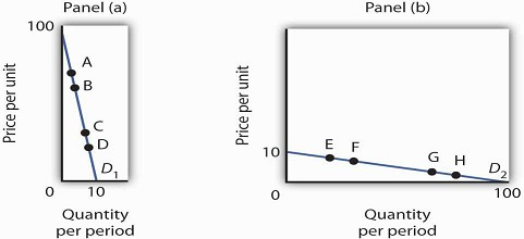
The table gives the prices and quantities corresponding to each of the points shown on the two demand curves.
|
Demand curve D1 [Panel (a)] |
Price | Quantity | |
|---|---|---|---|
|
A |
80 |
2 |
E |
|
B |
70 |
3 |
F |
|
C |
30 |
7 |
G |
|
D |
20 |
8 |
H |
- Suppose Janice buys the following amounts of various food items depending on her weekly income:
- Compute Janice’s income elasticity of demand for hamburgers.
- Compute Janice’s income elasticity of demand for pizza.
- Compute Janice’s income elasticity of demand for ice cream sundaes.
- Classify each good as normal or inferior.
|
Weekly Income |
Hamburgers |
Pizza |
Icecream |
|---|---|---|---|
|
$500 |
3 |
3 |
2 |
|
$750 |
4 |
2 |
2 |
- Suppose the following table describes Jocelyn’s weekly snack purchases, which vary depending on the price of a bag of chips:
- Compute the cross price elasticity of salsa with respect to the price of a bag of chips.
- Compute the cross price elasticity of pretzels with respect to the price of a bag of chips.
- Compute the cross price elasticity of soda with respect to the price of a bag of chips.
- Are chips and salsa substitutes or complements? How do you know?
- Are chips and pretzels substitutes or complements? How do you know?
- Are chips and soda substitutes or complements? How do you know?
|
Price of bag of chips |
Bags of chips |
Containers of salsa |
Bags of pretzels |
Cans of soda |
|---|---|---|---|---|
|
$1.00 |
2 |
3 |
1 |
4 |
|
$1.50 |
1 |
2 |
2 |
4 |
-
The table below describes the supply curve for light bulbs, compute the price elasticity of
supply and determine whether supply is price elastic, price inelastic, perfectly elastic, perfectly inelastic, or unit elastic:
- when the price of a light bulb increases from $1.00 to $1.50.
- when the price of a light bulb increases from $1.50 to $2.00.
- when the price of a light bulb increases from $2.00 to $2.50.
- when the price of a light bulb increases from $2.50 to $3.00.
| Price per light bulb | Quantity supplied |
|---|---|
| $1.00 | 500 |
| 1.50 | 3,000 |
| 2.00 | 4,000 |
| 2.50 | 4,500 |
| 3.00 | 4,500 |
ENDNOTES
- Notice that since the number of units sold of a good is the same as the number ofunits bought, the definition for total revenue could also be used to define total spending. Which term we use depends on the question at hand. If we are trying todetermine what happens to revenues of sellers, then we are asking about total revenue. If we are trying to determine how much consumers spend, then we are asking about total spending.
- Division by zero results in an undefined solution. Saying that the price elasticity of demand is infinite requires that we say the denominator “approaches” zero.
- See Georges Bresson, Joyce Dargay, Jean-Loup Madre, and Alain Pirotte, “Economic and Structural Determinants of the Demand for French Transport: An Analysis on a Panel of French Urban Areas Using Shrinkage Estimators.” Transportation Research:Part A 38: 4 (May 2004): 269–285. See also Anna Matas. “Demand and Revenue Implications of an Integrated Transport Policy: The Case of Madrid.” Transport Reviews24:2 (March 2004): 195–
- 217.
- Robert B. Ekelund, S. Ford, and John D. Jackson. “Are Local TV Markets Separate Markets?”International Journal of the Economics of Business 7:1 (2000): 79–97.
- Although close to zero in all cases, the significant and positive signs of income elasticityfor marijuana, alcohol, and cocaine suggest that they are normal goods, but significant and negative signs, in the case of heroin, suggest that heroin is an inferior good; Saffer and Chaloupka (cited below) suggest the effects of income for all four substances might be affected by education.
Sources: John A. Tauras. “Public Policy and Smoking Cessation among Young Adults in the United States,” Health Policy, 68:3 (June 2004): 321–332. Georges Bresson, Joyce Dargay, Jean-Loup Madre, and Alain Pirotte, “Economic and Structural Determinants of the Demand for French Transport: An Analysis on a Panel of French Urban Areas Using Shrinkage Estimators,” Transportation Research: Part A 38:4 (May 2004): 269–285; Avner Bar-Ilan and Bruce Sacerdote, “The Response of Criminals and Non-Criminals to Fines,” Journal of Law and Economics, 47:1 (April 2004): 1–17; Hana Ross and Frank J. Chaloupka, “The Effect of Public Policies and Prices on Youth Smoking,” Southern Economic Journal 70:4 (April 2004): 796–815; Anna Matas,“Demand and Revenue Implications of an Integrated Transport Policy: The Case of Madrid,” Transport Reviews, 24:2 (March 2004): 195–217; Matthew C. Farrelly, Terry F.Pechacek, and Frank J. Chaloupka; “The Impact of Tobacco Control Program Expenditures on Aggregate Cigarette Sales: 1981–2000,” Journal of Health Economics 22:5 (September 2003): 843–859; Robert B. Ekelund, S. Ford, and John D. Jackson. “Are Local TV Markets Separate Markets?” International Journal of the Economics of Business 7:1 (2000): 79–97; Henry Saffer and Frank Chaloupka, “The Demand for Illicit Drugs,Economic Inquiry 37(3) (July, 1999): 401– 411; Robert W. Fogel, “Catching Up With the Economy,” American Economic Review 89(1) (March, 1999):1–21; Michael Grossman,“A Survey of Economic Models of Addictive Behavior,” Journal of Drug Issues 28:3 (Summer 1998):631–643; Sanjib Bhuyan and Rigoberto A. Lopez, “Oligopoly Power inthe Food and Tobacco Industries,” American Journal of Agricultural Economics 79 (August 1997):1035–1043; Michael Grossman, “Cigarette Taxes,” Public Health Report 112:4 (July/August 1997): 290–297; Ann Hansen, “The Tax Incidence of the Colorado State Lottery Instant Game,” Public Finance Quarterly 23(3) (July, 1995):385–398 Daniel B. Suits, “Agriculture,” in Walter Adams and James Brock, eds., The Structure of American Industry, 9th ed. (Englewood Cliffs: Prentice Hall, , 1995), pp. 1–33; Kenneth G. Elzinga, “Beer,” in Walter Adams and James Brock, eds., The Structure of American Industry, 9th ed. (Englewood Cliffs: Prentice Hall, 1995), pp. 119–151; John A. Rizzo and David Blumenthal, “Physician Labor Supply: Do Income Effects Matter?” Journal of Health Economics 13(4) (December 1994):433–453; Douglas M. Brown, “The Rising Price of Physicians’ Services: A Correction and Extension on Supply,” Review of Economics and Statistics 76(2) (May 1994):389–393; George C. Davis and Michael K. Wohlgenant, “Demand Elasticities from a Discrete Choice Model: The Natural Christmas Tree Market,” Journal of Agricultural Economics 75(3) (August 1993):730–738; David M.Blau, “The Supply of Child Care Labor,” Journal of Labor Economics 2(11) (April 1993):324–347; Richard Blundell et al., “What Do We Learn About Consumer Demand Patterns from Micro Data?”, American Economic Review 83(3) (June 1993):570–597; F. Gasmi, et al., “Econometric Analysis of Collusive Behavior in a Soft-Drink Market,” Journal of Economics and Management Strategy (Summer 1992), pp. 277–311; M.R. Baye, D.W. Jansen, and J.W. Lee, “Advertising Effects in Complete Demand Systems,”Applied Economics 24 (1992):1087–1096; Gary
W. Brester and Michael K. Wohlgenant, “Estimating Interrelated Demands for Meats Using New Measures for Ground andTable Cut Beef,” American Journal of Agricultural Economics 73 (November 1991):1182–1194; Adesoji, O. Adelaja, “Price Changes, Supply Elasticities, Industry Organization,and Dairy Output Distribution,” American Journal of Agricultural Economics 73:1 (February 1991):89– 102; Mark A. R. Kleinman, Marijuana: Costs of Abuse, Costs of Control (NY:Greenwood Press, 1989); Jules M. Levine, et al., “The Demand for Higher Education in Three Mid-Atlantic States,” New York Economic Review 18 (Fall 1988):3–20; Dale Heien and Cathy Roheim Wessells, “The Demand for Dairy Products: Structure, Prediction, and Decomposition,” American Journal of Agriculture Economics(May 1988):219–228; Michael Grossman and Henry Saffer, “Beer Taxes, the Legal Drinking Age, and Youth Motor Vehicle Fatalities,” Journal of Legal Studies 16(2) (June1987):351– 374; James M. Griffin and Henry B. Steele, Energy Economics and Policy (New York: Academic Press, 1980), p. 232.
Dale M. Heien and Cathy Roheim Wessels, “The Demand for Dairy Products: Structure, Prediction, and Decomposition,” American Journal of Agricultural Economics 70:2(May 1988): 219–228.
David Romer, “Do Students Go to Class? Should They?” Journal of Economic Perspectives
- 3197 reads
