


As in the short run, costs in the long run depend on the firm’s level of output, the costs of factors, andthe quantities of factors needed for each level of output. The chief difference between long-and shortrun costs is there are no fixed factors in the long run. There are thus no fixed costs. All costs are variable,so we do not distinguish between total variable cost and total cost in the long run: total cost is total variable cost. The long-run average cost (LRAC) curve shows the firm’s lowest cost per unit at each level of output, assuming that all factors of production are variable. The LRAC curve assumes that the firm has chosen the optimal factor mix, as described in the previous section, for producing any level of output.The costs it shows are therefore the lowest costs possible for each level of output. It is important to note, however, that this does not mean that the minimum points of each short-run ATC curves lie onthe LRAC curve. This critical point is explained in the next paragraph and expanded upon even further in the next section. Figure 8.14 shows how a firm’s LRAC curve is derived. Suppose Lifetime Disc Co. produces compactdiscs (CDs) using capital and labor. We have already seen how a firm’s average total cost curve can be drawn in the short run for a given quantity of a particular factor of production, such as capital. In the short run, Lifetime Disc might be limited to operating with a given amount of capital; it would face one of the short-run average total cost curves shown in Figure 8.14. If it has 30 units of capital, for example,its average total cost curve is ATC30. In the long run the firm can examine the average total cost curves associated with varying levels of capital. Four possible short-run average total cost curves for Lifetime Disc are shown in Figure 8.14 for quantities of capital of 20, 30, 40, and 50 units. The relevantcurves are labeled ATC20, ATC30, ATC40, and ATC50 respectively. The LRAC curve is derived from this set of short-run curves by finding the lowest average total cost associated with each level of output.Again, notice that the U-shaped LRAC curve is an envelope curve that surrounds the various short-run ATC curves. With the exception of ATC40, in this example, the lowest cost per unit for a particular level of output in the long run is not the minimum point of the relevant short-run curve.
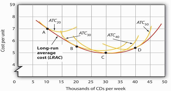
The LRAC curve is found by taking the lowest average total cost curve at each level of output. Here, average totalcost curves for quantities of capital of 20, 30, 40, and 50 units are shown for the Lifetime Disc Co. At a production level of 10,000 CDs per week, Lifetime minimizes its cost per CD by producing with 20 units of capital (point A). At 20,000 CDs per week, an expansion to a plant size associated with 30 units of capital minimizes cost per unit (pointB). The lowest cost per unit is achieved with production of 30,000 CDs per week using 40 units of capital (point C). If Lifetime chooses to produce 40,000 CDs per week, it will do so most cheaply with 50 units of capital (point D).
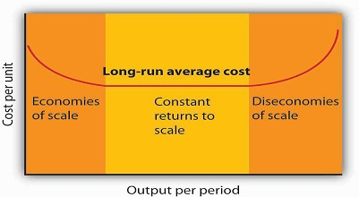
The downward-sloping region of the firm’sLRAC curve is associated with economies of scale. There may be a horizontal range associated with constant returns to scale. The upward-sloping range of the curve implies diseconomies of scale.
Economies and Diseconomies of Scale
Notice that the long-run average cost curve in Figure Figure 8.14 first slopes downward and then slopes upward.The shape of this curve tells us what is happening to average cost as the firm changes its scale of operations. A firm is said to experience economies of scale when long-run average cost declines as the firm expands its output. A firm is said to experience diseconomies of scale when long-run average cost increases as the firm expands its output. Constant returns to scale occur when long-run average cost stays the same over an output range.
Why would a firm experience economies of scale? One source of economies of scale is gains fromspecialization. As the scale of a firm’s operation expands, it is able to use its factors in more specialized ways, increasing their productivity. Another source of economies of scale lies in the economies that canbe gained from mass production methods. As the scale of a firm’s operation expands, the company can begin to utilize large-scale machines and production systems that can substantially reduce cost per unit.
Why would a firm experience diseconomies of scale? At first glance, it might seem that the answer lies in the law of diminishing marginal returns, but this is not the case. The law of diminishing marginal returns, after all, tells us how output changes as a single factor is increased, with all other factors ofproduction held constant. In contrast, diseconomies of scale describe a situation of rising average cost even when the firm is free to vary any or all of its factors as it wishes. Diseconomies of scale are generallythought to be caused by management problems. As the scale of a firm’s operations expands, it becomes harder and harder for management to coordinate and guide the activities of individual units of the firm. Eventually, the diseconomies of management overwhelm any gains the firm might be achieving by operating with a larger scale of plant, and long-run average costs begin rising. Firms experience constant returns to scale at output levels where there are neither economies nor diseconomies of scale.For the range of output over which the firm experiences constant returns to scale, the long-run average cost curve is horizontal.
Firms are likely to experience all three situations, as shown in Figure Figure 8.15. At very low levels of output, the firm is likely to experience economies of scale as it expands the scale of its operations. There may follow a range of output over which the firm experiences constant returns to scale— empirical studies suggest that the range over which firms experience constant returns to scale is often very large. And certainly there mustbe some range of output over which diseconomies of scale occur; this phenomenon is one factor that limits the size of firms. A firm operating on the upward-sloping part of its LRAC curve is likely to be undercut in the market by smaller firms operating with lower costs per unit of output.
The Size Distribution of Firms
Economies and diseconomies of scale have a powerful effect on the sizes of firms that will operate in any market. Suppose firms in a particular industry experience diseconomies of scale at relatively low levels of output. That industry will be characterized by a large number of fairly small firms. The restaurant market appears to be such an industry. Barbers and beauticians are another example.
If firms in an industry experience economies of scale over a very wide range of output,firms that expand to take advantage of lower cost will force out smaller firms that have higher costs. Such industries are likely to have a few large firms instead of many small ones. In the refrigerator industry, for example, the size of firm necessary toachieve the lowest possible cost per unit is large enough to limit the market to only a few firms. In most cities, economies of scale leave room for only a single newspaper.
One factor that can limit the achievement of economies of scale is the demand facing an individual firm. The scale of output required to achieve the lowest unit costs possible may require sales that exceed the demand facing a firm. A grocery store, for example, could minimize unitcosts with a large store and a large volume of sales. But the demand for groceries in a small, isolated community may not be able to sustain such a volume of sales. The firm is thus limited to a small scale of operation even though this might involve higher unit costs.
KEY TAKEAWAYS
- A firm chooses its factor mix in the long run on the basis of the marginal decision rule; it seeks to equate the ratio of marginal product to price for all factors of production. By doing so, it minimizes the cost of producing a given level of output.
- The long-run average cost (LRAC ) curve is derived from the average total cost curves associated with different quantities of the factor that is fixed in the short run. The LRAC curve shows the lowest cost per unit at which each quantity can be produced when all factors of production, including capital, are variable.
- A firm may experience economies of scale, constant returns to scale, or diseconomies of scale. Economies of scale imply a downward-sloping long-run average cost (LRAC ) curve. Constant returns to scale imply a horizontal LRAC curve. Diseconomies of scale imply an upward-sloping LRAC curve.
- A firm’s ability to exploit economies of scale is limited by the extent of market demand for its products.
- The range of output over which firms experience economies of scale, constant return to scale, or diseconomies of scale is an important determinant of how many firms will survive in a particular market.
TRY IT!
- Suppose Acme Clothing is operating with 20 units of capital and producing 9 units of output at an average total cost of $67, as shown in Figure 8.8. How much labor is it using?
- Suppose it finds that, with this combination of capital and labor, MPK/PK > MPL/PL. What adjustment willthe firm make in the long run? Why does it not make this same adjustment in the short run?
Case in Point: Telecommunications Equipment, Economies of Scale, and Outage Risk
© 2010 Jupiterimages Corporation
How big should the call switching equipment a major telecommunications company uses be? Having bigger machines results in economies of scale but also raises the risk of larger outages that
will affect more customers.
Verizon Laboratories economist Donald E. Smith examined both the economies of scale available from larger equipment and the greater danger of more widespread outages. He concluded that
companies should not use the largest machines available because of the outage danger and that they should not use the smallest size because that would mean forgoing the potential gains from
economies of scale of larger sizes.
Switching machines, the large computers that handle calls for telecommunications companies, come in four basic “port matrix sizes.” These are measured in terms of Digital Cross-Connects
(DCS’s). The four DCS sizes available are 6,000; 12,000; 24,000; and 36,000 ports. Different machine sizes are made with the same components and thus have essentially the same probability of
breaking down. Because larger machines serve more customers, however, a breakdown in a large machine has greater consequences for the company.
The costs of an outage have three elements. The first is lost revenue from calls that would otherwise have been completed. Second, the FCC requires companies to provide a credit of one month
of free service after any outage that lasts longer than one minute. Finally, an outage damages a company’s reputation and inevitably results in dissatisfied customers—some of whom may switch
to other companies.
But, there are advantages to larger machines. A company has a “portfolio” of switching machines. Having larger machines lowers costs in several ways. First, the initial acquisition of the
machine generates lower cost per call completed the greater the size of the machine. When the company must make upgrades to the software, having fewer—and larger—machines means fewer upgrades
and thus lower costs.
In deciding on matrix size companies should thus compare the cost advantages of a larger matrix with the disadvantages of the higher outage costs associated with those larger matrixes. Mr.
Smith concluded that the economies of scale outweigh the outage risks as a company expands beyond 6,000 ports but that 36,000 ports is “too big” in the sense that the outage costs outweigh
the advantage of the economies of scale. The evidence thus suggests that a matrix size in the range of 12,000 to 24,000 ports is optimal.
Source: Donald E. Smith, “How Big Is Too Big? Trading Off the Economies of Scale of Larger Telecommunications Network Elements Against the Risk of Larger Outages,” European Journal
of Operational Research, 173 (1) (August 2006): 299–312.
ANSWERS TO TRY IT ! PROBLEMS
- To produce 9 jackets, Acme uses 4 units of labor.
- In the long run, Acme will substitute capital for labor. It cannot make this adjustment in the short run, because its capital is fixed in the short run.
- 6238 reads
