


Because a monopolistically competitive firm faces a downward-sloping demand curve, its marginal revenue curve is a downward-sloping line that lies below the demand curve, as in the monopoly model. We can thus use the model of monopoly that we have already developed to analyze the choices of a monopsony in the short run.
Figure 11.1 shows the demand, marginal revenue, marginal cost, and average total cost curves facing a monopolistically competitive firm, Mama’s Pizza. Mama’s competes with several other similar firms in a market in which entry and exit are relatively easy. Mama’s demand curve D1 is downward sloping; even if Mama’s raises its prices above those of its competitors, it will still have some customers. Given the downward-sloping demand curve, Mama’s marginal revenue curve MR1 lies below demand. To sell more pizzas, Mama’s must lower its price, and that means its marginal revenue from additional pizzas will be less than price.
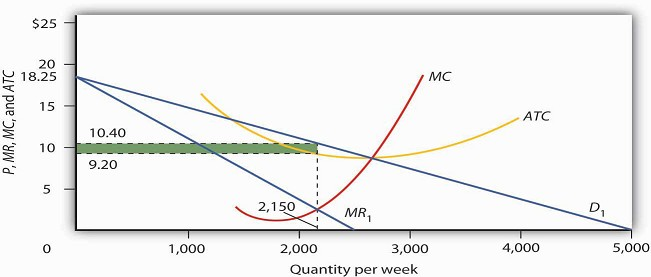
Looking at the intersection of the marginal revenue curve MR1 and the marginal cost curve MC, we see that the profit-maximizing quantity is 2,150 units per week. Reading up to the average total cost curve ATC, we see that the cost per unit equals $9.20. Price, given on the demand curve D1, is $10.40, so the profit per unit is $1.20. Total profit per week equals $1.20 times 2,150, or $2,580; it is shown by the shaded rectangle.
Given the marginal revenue curve MR and marginal cost curve MC, Mama’s will maximize profits by selling 2,150 pizzas per week. Mama’s demand curve tells us that it can sell that quantity at a price of $10.40. Looking at the average total cost curve ATC, we see that the firm’s cost per unit is $9.20. Its economic profit per unit is thus $1.20. Total economic profit, shown by the shaded rectangle, is $2,580 per week.
- 3542 reads
