


The amount that an additional unit of a factor adds to a firm’s total revenue during a period is called the marginal revenue product (MRP) of the factor. An additional unit of a factor of production adds to a firm’s revenue in a two-step process: first, it increases the firm’s output. Second, the increasedoutput increases the firm’s total revenue. We find marginal revenue product by multiplying the marginal product (MP) of the factor by the marginal revenue (MR).
EQUATION 12.1
MRP = MP × MR
In a perfectly competitive market the marginal revenue a firm receives equals the market-determined price P. Therefore, for firms in perfect competition, we can express marginal revenue product as follows:
EQUATION 12.2
In perfect competition, MRP = MP × P
The marginal revenue product of labor (MRPL) is the marginal product of labor (MPL) times the marginal revenue (which is the same as price under perfect competition) the firm obtains from additional units of output that result from hiring the additional unit of labor. If an additional worker adds 4 units of output per day to a firm’s production, and if each of those 4 units sells for $20, then the worker’s marginal revenue product is $80 per day. With perfect competition, the marginal revenue product for labor, MRPL, equals the marginal product of labor, MPL, times the price, P, of the good or service the labor produces:
EQUATION 12.3
In perfect competition, MRPL = MPL × P
The law of diminishing marginal returns tells us that if the quantity of a factor is increased while other inputs are held constant, its marginal product will eventually decline. If marginal product is falling, marginal revenue product must be falling as well.
Suppose that an accountant, Stephanie Lancaster, has started an evening call-in tax advisory service. Between the hours of 7 p.m. and 10 p.m., customers can call and get advice on their income taxes. Ms. Lancaster’s firm, TeleTax, is one of several firms offering similar advice; the going market price is $10 per call. Ms. Lancaster’s business has expanded, so she hires other accountants to handle the calls. She must determine how many accountants to hire.
As Ms. Lancaster adds accountants, her service can take more calls. The table in Figure 12.3 gives the relationship between the number of accountants available to answer calls each evening and the number of calls TeleTax handles. Panel (a) shows the increase in the number of calls handled by each additional accountant—that accountant’s marginal product. The first accountant can handle 13 calls per evening. Adding a second accountant increases the number of calls handled by 20. With two accountants, a degree of specialization is possible if each accountant takes calls dealing with questions about which he or she has particular expertise. Hiring the third accountant increases TeleTax’s output per evening by 23 calls.
Suppose the accountants share a fixed facility for screening and routing calls. They also share a stock of reference materials to use in answering calls. As more accountants are added, the firm will begin to experience diminishing marginal returns. The fourth accountant increases output by 20 calls.The marginal product of additional accountants continues to decline after that. The marginal product curve shown in Panel (a) of Figure 12.3 thus rises and then falls.
Each call TeleTax handles increases the firm’s revenues by $10. To obtain marginal revenue product, we multiply the marginal product of each accountant by $10; the marginal revenue product curve is shown in Panel (b) of Figure 12.3.
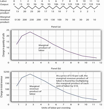
The table gives the relationship between the number of accountants employed by TeleTax each evening and the total number of calls handled. From these values we derive the marginal product and marginal revenue product curves.
We can use Ms. Lancaster’s marginal revenue product curve to determine the quantity of labor she will hire. Suppose accountants in her area are available to offer tax advice for a nightly fee of $150. Each additional accountant Ms. Lancaster hires thus adds $150 per night to her total cost. The amount a factor adds to a firm’s total cost per period is called its marginal factor cost (MFC). Marginal factor cost (MFC) is the change in total cost (ΔTC) divided by the change in the quantity of the factor (Δf):
EQUATION 12.4
The marginal factor cost to TeleTax of additional accountants ($150 per night) is shown as a horizontal line in Figure 12.4. It is simply the market wage (i.e., the price per unit of labor).
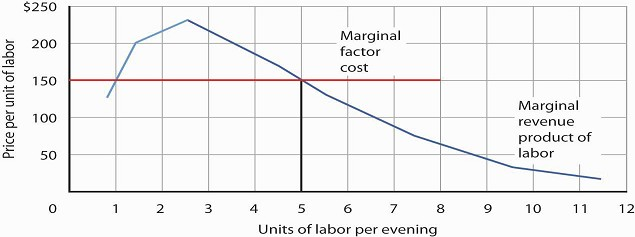
The downward-sloping portion of a firm’s marginal revenue product curve is its demand curve for a variable factor. At a marginal factor cost of $150, TeleTax hires the services of five accountants.
TeleTax will maximize profit by hiring additional units of labor up to the point where the downwardsloping portion of the marginal revenue product curve intersects the marginal factor cost curve; we see in Figure Figure 12.3 that it will hire five accountants. Based on the information given in the table in Figure Figure 12.2, we know that the five accountants will handle a total of 93 calls per evening; TeleTax will earn total revenue of $930 per evening. The firm pays $750 for the services of the five accountants—that leaves $180 to apply to the fixed cost associated with the tax advice service and the implicit cost ofStephanie Lancaster’s effort in organizing the service. Recall that these implicit costs include the income forgone (that is, opportunity cost) by not shifting her resources, including her own labor, to her next best alternative.
If TeleTax had to pay a higher price for accountants, it would face a higher marginal factor cost curve and would hire fewer accountants. If the price were lower, TeleTax would hire more accountants.The downward-sloping portion of TeleTax’s marginal revenue product curve shows the number of accountants it will hire at each price for accountants; it is thus the firm’s demand curve for accountants.It is the portion of the curve that exhibits diminishing returns, and a firm will always seek to operate in the range of diminishing returns to the factors it uses.
It may seem counterintuitive that firms do not operate in the range of increasing returns, which would correspond to the upward-sloping portion of the marginal revenue product curve. However, to do so would forgo profit-enhancing opportunities. For example, in Figure Figure 12.4, adding the second accountantadds $200 to revenue but only $150 to cost, so hiring that accountant clearly adds to profit.But why stop there? What about hiring a third accountant? That additional hire adds even more to revenue ($230) than to cost. In the region of increasing returns, marginal revenue product rises. With marginal factor cost constant, not to continue onto the downward-sloping part of the marginal revenue curve would be to miss out on profit-enhancing opportunities. The firm continues adding accountants until doing so no longer adds more to revenue than to cost, and that necessarily occurs where the marginal revenue product curve slopes downward.
In general, then, we can interpret the downward-sloping portion of a firm’s marginal revenue product curve for a factor as its demand curve for that factor. 1 We find the market demand for labor by adding the demand curves for individual firms.
Heads Up!
The Two Rules Lead to the Same Outcome
In the chapter on competitive output markets we learned that profit-maximizing firms will increase output so long as doing so adds more to revenue than to cost, or up to the point where marginal revenue, which in perfect competition is the same as the market-determined price, equals marginal cost. In this chapter we have learned that profit-maximizing firms will hire labor up to the point where marginal revenue product equals marginal factor cost. Is it possible that a firm that follows the marginal decision rule for hiring labor would end up producing a different quantity of output compared to the quantity of output it would choose if it followed the marginal decision rule for deciding directly how much output to produce? Is there a conflict between these two marginal decision rules? The answer is no. These two marginal decision rules are really just two ways of saying the same thing: one rule is in terms of quantity of output and the other in terms of the quantity of factors required to produce that quantity of output. Hiring an additional unit of a factor means producing a certain amount of additional output.
Using the example of TeleTax, at $150 per accountant per night, we found that Ms. Lancaster maximizes profit by hiring five accountants. The MPL of the fifth accountant is ΔQ; it is 17. At five accountants, the marginal cost of a call is ΔTC / ΔQ = $150 / 17 = $8.82 , which is less than the price of $10 per call, so hiring that accountant adds to her profit. At six accountants, the marginal cost of a call would be $150 / 13 = $11.54 , which is greater than the $10 price, so hiring a sixth accountant would lower profit. The profit-maximizing output of 93 calls, found by comparing marginal cost and price, is thus consistent with the profit-maximizing quantity of labor of five accountants, found by comparing marginal revenue product and marginal factor cost.
- 11589 reads
