


Monopsony power may also exist in markets for factors other than labor. The military in different countries, for example, has considerable monopsony power in the market for sophisticated military goods. Major retailers often have some monopsony power with respect to some of their suppliers.Sears, for example, is the only wholesale buyer of Craftsman brand tools. One major development in medical care in recent years has been the emergence of managed care organizations that contract with a large number of employers to purchase medical services on behalf of employees. These organizations often have sufficient monopsony power to force down the prices charged by providers such as drug companies, physicians, and hospitals. Countries in which health care is provided by the government, such as Canada and the United Kingdom, are able to exert monopsony power in their purchase of health care services.
Whatever the source of monopsony power, the expected result is the same. Buyers with monopsony power are likely to pay a lower price and to buy a smaller quantity of a particular factor than buyers who operate in a more competitive environment.
KEY TAKEAWAYS
- In the monopsony model there is one buyer for a good, service, or factor of production. A monopsony firm is a price setter in the market in which it has monopsony power.
- The monopsony buyer selects a profit-maximizing solution by employing the quantity of factor at which marginal factor cost (MFC) equals marginal revenue product (MRP) and paying the price on the factor’s supply curve corresponding to that quantity.
- A degree of monopsony power exists whenever a firm faces an upward-sloping supply curve for a factor.
TRY IT!
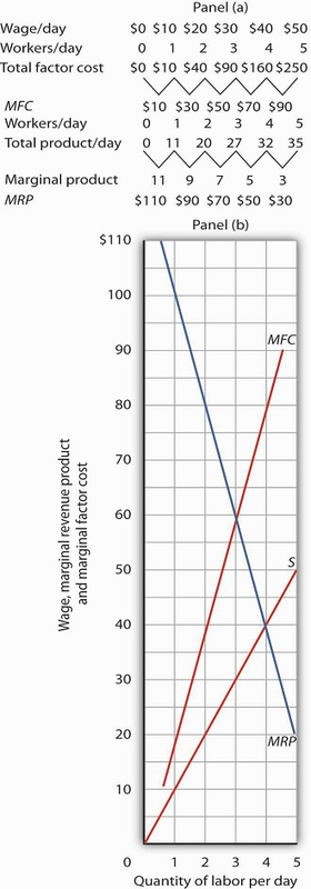
Suppose a firm is the only employer of labor in an isolated area and faces the supply curve for labor suggested by the following table. Plot the supply curve. To compute the marginal factor
cost curve, compute total factor cost and then the values for the marginal factor cost curve (remember to plot marginal values at the midpoints of the respective intervals). (Hint: follow the
example of Figure 14.2.) Compute MRP and plot the MRP curve on the same graph on which you have plotted supply and MFC.
Now suppose you are given the following data for the firm’s total product at each quantity of labor. Compute marginal product. Assume the firm sells its product for $10 per unit in a
perfectly competitive market. Compute MRP and plot the MRP curve on the same graph on which you have plotted supply and MFC. Remember to plot marginal values at the midpoints of the
respective axes.
How much labor will the firm employ? What wage will it pay?
Case in Point: Professional Player Salaries and Monopsony
Professional athletes have not always enjoyed the freedom they have today to seek better offers from other teams. Before 1977, for example, baseball players could deal only with the team that
owned their contract— one that “reserved” the player to that team. This reserve clause gave teams monopsony power over the players they employed. Similar restrictions hampered player mobility
in men’s football, basketball, and hockey.
Gerald Scully, an economist at the University of Texas at Dallas, estimated the impact of the reserve clause on baseball player salaries. He sought to demonstrate that the player salaries
fell short of MRP. Mr. Scully estimated the MRP of players in a two-step process. First, he studied the determinants of team attendance. He found that in addition to factors such as
population and income in a team’s home city, the team’s win-loss record had a strong effect on attendance. Second, he examined the player characteristics that determined winloss records. He
found that for hitters, batting average was the variable most closely associated with a team’s winning percentage. For pitchers, it was the earned-run average—the number of earned runs
allowed by a pitcher per nine innings pitched.
With equations that predicted a team’s attendance and its win-loss record, Mr. Scully was able to take a particular player, describe him by his statistics, and compute his MRP. Mr. Scully
then subtracted costs associated with each player for such things as transportation, lodging, meals, and uniforms to obtain the player’s net MRP. He then compared players’ net MRPs to their
salaries.
Mr. Scully’s results, displayed in the table below, show net MRP and salaries, estimated on a career basis, for players he classified as mediocre, average, and star-quality, based on their
individual statistics. For average and star-quality players, salaries fell far below net MRP, just as the theory of monopsony suggests.
|
Career Net MRP |
Career Salary |
|
|---|---|---|
|
Hitters |
||
|
Mediocre |
-$129,300 |
$60,800 |
|
Average |
90,700 |
196,200 |
|
Star |
3,139,100 |
477,200 |
|
Pitchers |
||
|
Mediocre |
-53,600 |
54,800 |
|
Average |
1,119,200 |
222,500 |
|
Star |
3,969,600 |
612,500 |
The fact that mediocre players with negative net MRPs received salaries presents something of a puzzle. One explanation could be that when they were signed to contracts, these players were
expected to perform well, so their salaries reflected their expected contributions to team revenues. Their actual performance fell short, so their wages exceeded their MRPs. Another
explanation could be that teams paid young players more than they were expected to contribute to revenues early in their careers in hopes that they would develop into profitable members of
the team. In any event, Mr. Scully found that the costs of mediocre players exceeded their estimated contribution to team revenues, giving them negative net MRPs.
In 1977, a lawsuit filed by several baseball players resulted in the partial dismantling of the reserve clause. Players were given the right, after six years with a team, to declare
themselves “free agents” and offer their services to other teams. Player salaries quickly rose. The accompanying table shows the pitchers that became free agents in 1977, their estimated net
marginal revenue products, and their 1977 salaries. As you can see, salaries for pitchers came quite close to their net MRPs.
|
Pitcher |
Net MRP |
1977 Salary |
|---|---|---|
|
Doyle Alexander |
$166,203 |
$166,677 |
|
Bill Campbell |
$205,639 |
$210,000 |
|
Rollie Fingers |
$303,511 |
$332,000 |
|
Wayne Garland |
$282,091 |
$230,000 |
|
Don Gullett |
$340,846 |
$349,333 |
The same movement toward giving players greater freedom to deal with other teams occurred in the National Football League (NFL), the National Basketball Association (NBA), and the National
Hockey League (NHL). The result in every case was the same: player salaries rose both in absolute terms and as a percentage of total team revenues. Table 14.1 gives player salaries as a
percentage of total team revenues in the period 1970–73 and in 1998 for men’s baseball (MLB), basketball, football, and hockey.
The greatest gains came in baseball, which had the most restrictive rules against player movement. Hockey players, too, ended up improving their salaries greatly. By 2004, their salaries
totaled 75% of team revenues. The smallest gains came in basketball, where players already had options. The American Basketball Association was formed; it ultimately became part of the
National Basketball Association. Basketball players also had the alternative of playing in Europe. But, the economic lesson remains clear: any weakening of the monopsony power of teams
results in gains in player salaries.
Sources: Gerald Scully, “Pay and Performance in Major League Baseball,” American Economic Review, 64 (2) (December 1974): 915–30. Gerald W. Scully, “Player Salary Share and the Distribution
of Player Earnings,” Managerial and Decision Economics, 25 (2004): 77–86.
ANSWER TO TRY IT! PROBLEM
The completed tables are shown in Panel (a). Drawing the supply (S), MFC, and MRP curves, we have Panel (b). The monopsony firm will employ three units of labor per day (the quantity at which MRP = MFC ) and will pay a wage taken from the supply curve: $30 per day.
- 2612 reads
