


In each of the models of market failure we have reviewed here—public goods, external costs and benefits, and imperfect competition—the market may fail to achieve the efficient result. There is a potential for government intervention to move inefficient markets closer to the efficient solution.
Figure 15.3 reviews the potential gain from government intervention in cases of market failure. In each case, the potential gain is the deadweight loss resulting from market failure; government intervention may prevent or limit this deadweight loss. In each panel, the deadweight loss resulting from market failure is shown as a shaded triangle.
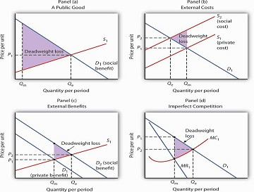
In each panel, the potential gain from government intervention to correct market failure is shown by the deadweight loss avoided, as given by the shaded triangle. In Panel (a), we assume that a private market produces Qm units of a public good. The efficient level, Qe, is defined by the intersection of the demand curve D1 for the public good and the supply curve S1. Panel (b) shows that if the production of a good generates an external cost, the supply curve S1 reflects only the private cost of the good. The market will produce Qm units of the good at price P1. If the public sector finds a way to confront producers with the social cost of their production, then the supply curve shifts to S2, and production falls to the efficient level Qe. Notice that this intervention results in a higher price, P2, which confronts consumers with the real cost of producing the good. Panel (c) shows the case of a good that generates external benefits. Purchasers of the good base their choices on the private benefit, and the market demand curve is D1. The market quantity is Qm. This is less than the efficient quantity, Qe, which can be achieved if the activity that generates external benefits is subsidized. That would shift the market demand curve to D2, which intersects the market supply curve at the efficient quantity. Finally, Panel (d) shows the case of a monopoly firm that produces Qm units and charges a price P1. The efficient level of output, Qe, could be achieved by imposing a price ceiling at P2. As is the case in each of the other panels, the potential gain from such a policy is the elimination of the deadweight loss shown as the shaded area in the exhibit.
Panel (a) of Figure 15.3 illustrates the case of a public good. The market will produce some of the public good; suppose it produces the quantity Qm. But the demand curve that reflects the social benefits ofthe public good, D1, intersects the supply curve at Qe; that is the efficient quantity of the good. Public sector provision of a public good may move the quantity closer to the efficient level.
Panel (b) shows a good that generates external costs. Absent government intervention, these costs will not be reflected in the market solution. The supply curve, S1, will be based only on the private costs associated with the good. The market will produce Qm units of the good at a price P1. If the government were to confront producers with the external cost of the good, perhaps with a tax on the activity that creates the cost, the supply curve would shift to S2 and reflect the social cost of the good. The quantity would fall to the efficient level, Qe, and the price would rise to P2.
Panel (c) gives the case of a good that generates external benefits. The demand curve revealed in the market, D1, reflects only the private benefits of the good. Incorporating the external benefits of the good gives us the demand curve D2 that reflects the social benefit of the good. The market’s output of Qm units of the good falls short of the efficient level Qe.
The government may seek to move the market solution toward the efficient level through subsidies or other measures to encourage the activity that creates the external benefit.
Finally, Panel (d) shows the case of imperfect competition. A firm facing a downward-sloping demand curve such as D1 will select the output Qm at which the marginal cost curve MC1 intersects the marginal revenue curve MR1. The government may seek to move the solution closer to the efficient level, defined by the intersection of the marginal cost and demand curves.
While it is important to recognize the potential gains from government intervention to correct market failure, we must recognize the difficulties inherent in such efforts. Government officials may lack the information they need to select the efficient solution. Even if they have the information, they may have goals other than the efficient allocation of resources. Each instance of government intervention involves an interaction with utility-maximizing consumers and profit-maximizing firms, none of whom can be assumed to be passive participants in the process. So, while the potential exists for improved resource allocation in cases of market failure, government intervention may not always achieve it.
The late George Stigler, winner of the Nobel Prize for economics in 1982, once remarked that people who advocate government intervention to correct every case of market failure reminded him of the judge at an amateur singing contest who, upon hearing the first contestant, awarded first prize to the second. Stigler’s point was that even though the market is often an inefficient allocator of resources, so is the government likely to be. Government may improve on what the market does; it can also make it worse. The choice between the market’s allocation and an allocation with government intervention is always a choice between imperfect alternatives. We will examine the nature of public sector choices later in this chapter and explore an economic explanation of why government intervention may fail to move market solutions closer to their efficient levels.
- 3545 reads
