


The efficient level of pollution is the quantity at which its total benefits exceed its total costs by the greatest possible amount. This occurs where the marginal benefit of an additional unit of pollution equals its marginal cost.
Figure 18.1 shows how we can determine an efficient quantity of pollution. Suppose two neighbors in a remote mountain area, Mary and Jane, burn fires in their cabins that generate air pollution that harms two other individuals, Sam and Richard, who live downwind. We shall assume that Mary and Jane are the only polluters and that Sam and Richard are the only people harmed by the pollution. We shall ignore, for example, the effect of Mary and Jane’s emissions on the possible problem of global warming.
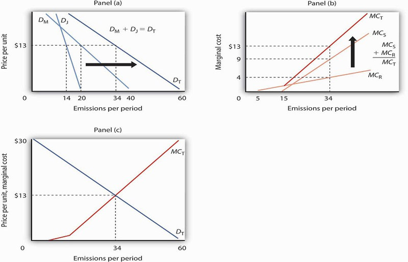
Mary and Jane each benefit from polluting the environment by emitting smoke from their fires. In Panel (a), we see that Mary’s demand curve for emitting smoke is given by DM and that Jane’s demand curve is given by DJ. To determine the total demand curve, DT, we determine the amount that each person will emit at various prices. At a price of $13 per day, for example, Mary will emit 20 pounds per day. Jane will emit 14 pounds per day, for a total of 34 pounds per day on demand curve DT. Notice that if the price were $0 per unit, Mary would emit 40 pounds per day, Jane would emit 20, and emissions would total 60 pounds per day on curve DT. The marginal cost curve for pollution is determined in Panel (b) by taking the marginal cost curves for each person affected by the pollution. In this case, the only people affected are Sam and Richard. Sam’s marginal cost curve is MCS, and Richard’s marginal cost curve is MCR. Because Sam and Richard are each affected by the same pollution, we add their marginal cost curves vertically. For example, if the total quantity of the emissions is 34 pounds per day, the marginal cost of the 34th pound to Richard is $4, it is $9 to Sam, for a total marginal cost of the 34th unit of $13. In Panel (c), we put DT and MCT together to find the efficient solution. The two curves intersect at a level of emissions of 34 pounds per day, which occurs at a price of $13 per pound.
Suppose, as is often the case, that no mechanism exists to charge Mary and Jane for their emissions; they can pollute all they want and never have to compensate society (that is, pay Sam and Richard) for the damage they do. Alternatively, suppose there is no mechanism for Sam and Richard to pay Mary and Jane to get them to reduce their pollution. In either situation, the pollution generated by Mary and Jane imposes an external cost on Sam and Richard. Mary and Jane will pollute up to the point that the marginal benefit of additional pollution to them has reached zero—that is, up to the point where the marginal benefit matches their marginal cost. They ignore the external costs they impose on “society”—Sam and Richard.
Mary’s and Jane’s demand curves for pollution are shown in Panel (a). These demand curves, DM and DJ, show the quantities of emissions each generates at each possible price, assuming such a fee were assessed. At a price of $13 per unit, for example, Mary will emit 20 units of pollutant per period and Jane will emit 14. Total emissions at a price of $13 would be 34 units per period. If the price of emissions were zero, total emissions would be 60 units per period. Whatever the price they face, Mary and Jane will emit additional units of the pollutant up to the point that their marginal benefit equals that price. We can therefore interpret their demand curves as their marginal benefit curves for emissions.
Their combined demand curve DT gives the marginal benefit to society (that is, to Mary and Jane) of pollution. Each person in our problem, Mary, Jane, Sam, and Richard, follows the marginal decision rule and thus attempts to maximize utility.
In Panel (b) we see how much Sam and Richard are harmed; the marginal cost curves, MCS and MCR, show their respective valuations of the harm imposed on them by each additional unit of emissions. Notice that over a limited range, some emissions generate no harm. At very low levels, neither Sam nor Richard is even aware of the emissions. Richard begins to experience harm as the quantity of emissions goes above 5 pounds per day; it is here that pollution begins to occur. As emissions increase, the additional harm each unit creates becomes larger and larger—the marginal cost curves are upward sloping. The first traces of pollution may be only a minor inconvenience, but as pollution goes up, the problems it creates become more serious—and its marginal cost rises.
Because the same emissions affect both Sam and Richard, we add their marginal cost curves vertically to obtain their combined marginal cost curve MCT. The 34th unit of emissions, for example, imposes an additional cost of $9 on Sam and $4 on Richard. It thus imposes a total marginal cost of $13. The efficient quantity of emissions is found at the intersection of the demand (DT) and marginal cost (MCT) curves in Panel (c) of Figure 18.1, with 34 units of the pollutant emitted. The marginal benefit of the 34th unit of emissions, as measured by the demand curve DT, equals its marginal cost, MCT, at that level. The quantity at which the marginal benefit curve intersects the marginal cost curve maximizes the net benefit of an activity.
We have already seen that in the absence of a mechanism to charge Mary and Jane for their emissions, they face a price of zero and would emit 60 units of pollutant per period. But that level of pollution is inefficient. Indeed, as long as the marginal cost of an additional unit of pollution exceeds its marginal benefit, as measured by the demand curve, there is too much pollution; the net benefit of emissions would be greater with a lower level of the activity.
Just as too much pollution is inefficient, so is too little. Suppose Mary and Jane are not allowed to pollute; emissions equal zero. We see in Panel (c) that the marginal benefit of dumping the first unit of pollution is quite high; the marginal cost it imposes on Sam and Richard is zero. Because the marginal benefit of additional pollution exceeds its marginal cost, the net benefit to society would be increased by increasing the level of pollution. That is true at any level of pollution below 34 units, the efficient solution.
The notion that too little pollution could be inefficient may strike you as strange. To see the logic of this idea, imagine that the pollutant involved is carbon monoxide, a pollutant emitted whenever combustion occurs, and it is deadly. It is, for example, emitted when you drive a car. Now suppose that no emissions of carbon monoxide are allowed. Among other things, this would require a ban on all driving. Surely the benefits of some driving would exceed the cost of the pollution created. The problem in pollution policy from an economic perspective is to find the quantity of pollution at which total benefits exceed total costs by the greatest possible amount—the solution at which marginal benefit equals marginal cost.
- 12377 reads
