


Pollutants harm people and the resources they value. The marginal cost curve for a pollutant shows the additional cost imposed by each unit of the pollutant. As we saw in Figure 18.1, the marginal cost curves for all the individuals harmed by a particular pollutant are added vertically to obtain the marginal cost curve for the pollutant.
Like the marginal benefit curve for emissions, the marginal cost curve can be interpreted in two ways, as suggested in Figure 18.3. When read from left to right, the curve measures the marginal cost of additional units of emissions (MCE). If increasing the motorists’ emissions from four pounds of carbon monoxide per week to five pounds of carbon monoxide per week imposes an external cost of $2, though, the marginal benefit of not being exposed to that unit of pollutant must be $2. The marginal cost curve can thus be read from right to left as a marginal benefit curve for abating emissions (MBA). This marginal benefit curve is, in effect, the demand curve for cleaner air.
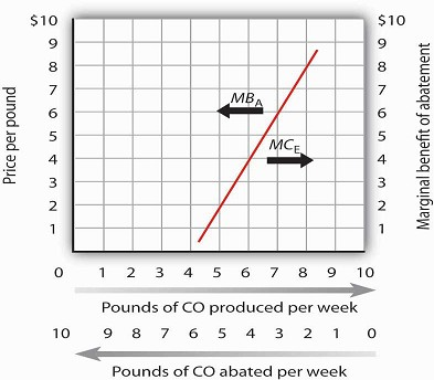
The marginal cost of the first few units of emissions is zero and then rises once emissions begin to harm people. That is the point at which the air becomes a scarce resource. Read from left to right the curve gives the marginal cost of emissions (MCE). Read from right to left, the curve gives the marginal benefit of abatement (MBA).
Economists estimate the marginal cost curve of pollution in several ways. One is to infer it from the demand for goods for which environmental quality is a complement. Another is to survey people, asking them what pollution costs—or what they would pay to reduce it. Still another is to determine the costs of damages created by pollution directly.
For example, environmental quality is a complement of housing. The demand for houses in areas with cleaner air is greater than the demand for houses in areas that are more polluted. By observing the relationship between house prices and air quality, economists can learn the value people place on cleaner air—and thus the cost of dirtier air. Studies have been conducted in cities all over the world to determine the relationship between air quality and house prices so that a measure of the demand for cleaner air can be made. They show that increased pollution levels result in lower house values. 1
Surveys are also used to assess the marginal cost of emissions. The fact that the marginal cost of an additional unit of emissions is the marginal benefit of avoiding the emissions suggests that surveys can be designed in two ways. Respondents can be asked how much they would be harmed by an increase in emissions, or they can be asked what they would pay for a reduction in emissions. Economists often use both kinds of questions in surveys designed to determine marginal costs.
A third kind of cost estimate is based on objects damaged by pollution. Increases in pollution, for example, require buildings to be painted more often; the increased cost of painting is one measure of the cost of added pollution.
While all of the attempts to measure cost are imperfect, the alternative is to not try to quantify cost at all. To economists, such an ostrich-like approach of sticking one’s head in the sand would be unacceptable.
The Efficient Level of Emissions and Abatement
Whether economists measure the marginal benefits and marginal costs of emissions or, alternatively, the marginal benefits and marginal costs of abatement, the policy implications are the same from an economic perspective. As shown in Panel (a) of Figure 18.4, applying the marginal decision rule in the case of emissions suggests that the efficient level of pollution occurs at six pounds of CO emitted per week. At any lower level, the marginal benefits of the pollution would outweigh the marginal costs. At a higher level, the marginal costs of the pollution would outweigh the marginal benefits.
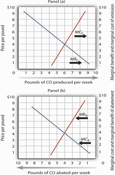
In Panel (a) we combine the marginal benefit of emissions (MBE) with the marginal cost of emissions (MCE). The efficient solution occurs at the intersection of the two curves. Here, the efficient quantity of emissions is six pounds of CO per week. In Panel (b), we have the same curves read from right to left. The marginal cost curve for emissions becomes the marginal benefit of abatement (MBA). The marginal benefit curve for emissions becomes the marginal cost of abatement (MCA). With no abatement program, emissions total ten pounds of CO per week. The efficient degree of abatement is to reduce emissions by four pounds of CO per week to six pounds per week.
As shown in Panel (b) of Figure 18.4, application of the marginal decision rule suggests that the efficient level of abatement effort is to reduce pollution by 4 pounds of CO produced per week. That is, reduce the level of pollution from the 10 pounds per week that would occur at a zero price to 6 pounds per week. For any greater effort at abating the pollution, the marginal cost of the abatement efforts would exceed the marginal benefit.
KEY TAKEAWAYS
- Pollution is related to the concept of scarcity. The existence of pollution implies that an environmental resource has alternative uses and is thus scarce.
- Pollution has benefits as well as costs; the emission of pollutants benefits people by allowing other activities to be pursued at lower costs. The efficient rate of emissions occurs where the marginal benefit of emissions equals the marginal cost they impose.
- The marginal benefit curve for emitting pollutants can also be read from right to left as the marginal cost of abating emissions. The marginal cost curve for increased emission levels can also be read from right to left as the demand curve for improved environmental quality.
- The Coase theorem suggests that if property rights are well-defined and if transactions are costless, then the private market will reach an efficient solution. These conditions, however, are not likely to be present intypical environmental situations. Even if such conditions do not exist, Coase’s arguments still yield useful insights to the mitigation of environmental problems.
- Surveys are sometimes used to measure the marginal benefit curves for emissions and the marginal cost curves for increased pollution levels. Marginal cost curves may also be inferred from other relationships. Two that are commonly used are the demand for housing and the relationship between pollution and production.
TRY IT!
The table shows the marginal benefit to a paper mill of polluting a river and the marginal cost to residents who live downstream. In this problem assume that the marginal benefits and
marginal costs are measured at (not between) the specific quantities shown.
Plot the marginal benefit and marginal cost curves. What is the efficient quantity of pollution? Explain why neither one ton nor five tons is an efficient quantity of pollution. In the
absence of pollution fees or taxes, how many units of pollution do you expect the paper mill will choose to produce? Why?
|
Quantity of pollution (tons per week) |
Marginal benefit |
Marginal cost |
|---|---|---|
|
0 |
$110 |
$0 |
|
1 |
100 |
8 |
|
2 |
90 |
20 |
|
3 |
80 |
35 |
|
4 |
70 |
70 |
|
5 |
60 |
150 |
|
6 |
0 |
300 |
Case in point: Estimating a Demand Curve for Environmental Quality
How do economists estimate demand curves for environmental quality? One recent example comes from work by Louisiana State University economist David M. Brasington and Auburn University
economist Diane Hite. Using data from Ohio’s six major metropolitan areas (Akron, Cincinnati, Cleveland, Columbus, Dayton, and Toledo), the economists studied the relationship between house
prices and the distance between individual houses and hazardous waste sites. From this, they were able to estimate the demand curve for environmental quality—at least in terms of the demand
for locations farther from environmental hazards.
The economists used actual real estate transactions in 1991 to get data on house prices. In that year, there were 1,192 hazardous sites in the six metropolitan areas. The study was based on
44,255 houses. The median distance between a house and a hazardous site was 1.08 miles. The two economists found, as one would expect, that house prices were higher the greater the distance
between the house and a hazardous site. All other variables unchanged, increasing the distance from a house to a hazardous site by 10% increased house value by 0.3%.
Other characteristics of the demand curve shed light on the relationship between environmental quality and other goods. For example, the study showed that people substitute house size for
environmental quality. A house closer to a hazardous waste site is cheaper; people take advantage of the lower price of such sites to purchase larger houses.
While house size and environmental quality were substitutes, school quality, measured by student scores on achievement tests, was a complement. If the price of school quality were to fall by
10%, household would buy 8% more environmental quality. The cross-price elasticity between environmental quality and school quality was thus estimated to be −0.80.
There is no marketplace for environmental quality. Estimating the demand curve for such quality requires economists to examine other data to try to infer what the demand curve is. The study
by Professors Brasington and Hite illustrates the use of an examination of an actual market, the market for houses, to determine characteristics of the demand curve for environmental
quality.
Source: David M. Brasington and Diane Hite, “Demand for Environmental Quality: A Spatial Hedonic Analysis,” Regional Science & Urban Economics, 35(1) (January 2005): 57–82.
ANSWER TO TRY IT ! PROBLEM
The efficient quantity of pollution is four tons per week. At one ton of pollution, the marginal benefit exceeds the marginal cost. If the paper mill expands production, the additional
pollution generated leads to additional benefits for it that are greater than the additional cost to the residents nearby. At five tons, the marginal cost of polluting exceeds the marginal
benefit. Reducing production, and hence pollution, brings the marginal costs and benefits closer.
In the absence of any fees, taxes, or other charges for its pollution, the paper mill will likely choose to generate six tons per week, where the marginal benefit has fallen to zero.

- 4041 reads
