


The primary evidence of growing inequality is provided by census data. Households are asked to report their income, and they are ranked from the household with the lowest income to the household with the highest income. The Census Bureau then reports the percentage of total income earned by those households ranked among the bottom 20%, the next 20%, and so on, up to the top 20%. Each 20% of households is called a quintile. The bureau also reports the share of income going to the top 5% of households.
Income distribution data can be presented graphically using a Lorenz curve, a curve that shows cumulative shares of income received by individuals or groups. It was developed by economist Max O.Lorenz in 1905. To plot the curve, we begin with the lowest quintile and mark a point to show the percentage of total income those households received. We then add the next quintile and its share and mark a point to show the share of the lowest 40% of households. Then, we add the third quintile, and then the fourth. Since the share of income received by all the quintiles will be 100%, the last point on the curve always shows that 100% of households receive 100% of the income.
If every household in the United States received the same income, the Lorenz curve would coincide with the 45-degree line drawn in Figure Figure 19.1. The bottom 20% of households would receive 20% of income; the bottom 40% would receive 40%, and so on. If the distribution of income were completely unequal, with one household receiving all the income and the rest zero, then the Lorenz curve would be shaped like a backward L, with a horizontal line across the bottom of the graph at 0% of income and a vertical line up the right-hand side. The vertical line would show, as always, that 100% of families still receive 100% of income. Actual Lorenz curves lie between these extremes. The closer a Lorenz curve lies to the 45-degree line, the more equal the distribution. The more bowed out the curve, the less equal the distribution. We see in Figure Figure 19.1 that the Lorenz curve for the United States became more bowed out between 1968 and 2006.
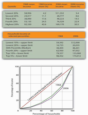
The distribution of income among households in the United States became more unequal from 1968 to 2006. The shares of income received by each of the first four quintiles fell, while the share received by the top 20% rose sharply. The Lorenz curve for 2006 was more bowed out than was the curve for 1968. (Mean income adjusted for inflation and reported in 2006 dollars; percentages do not sum to 100% due to rounding.)
Sources: Carmen DeNavas-Walt, Bernadette D. Proctor, and Cheryl Hill Lee, U.S. Census Bureau,
Current Population Reports, P60-229, Income, Poverty, and Health Insurance Coverage in the United States: 2004, U.S. Government Printing Office, Washington, DC, 2005, Table A-3; U.S. Census Bureau, Current Population Survey, 2005 Annual Social and Economic Supplement, Table HINC-05.
The degree of inequality is often measured with a Gini coefficient, the ratio between the Lorenz curve and the 45° line and the total area under the 45° line. The smaller the Gini coefficient, the more equal the income distribution. Larger Gini coefficients mean more unequal distributions. The Census Bureau reported that the Gini coefficient was 0.397 in 1968 and 0.470 in 2006—the highest ever recorded for the United States.
- 1893 reads
