


It seems reasonable to expect that consumption spending by households will be closely related to their disposable personal income, which equals the income households receive less the taxes they pay. Note that disposable personal income and GDP are not the same thing. GDP is a measure of total income; disposable personal income is the income households have available to spend during a specified period.
Real values of disposable personal income and consumption per year from 1960 through 2008 are plotted in Figure 28.1. The data suggest that consumption generally changes in the same direction as does disposable personal income.
The relationship between consumption and disposable personal income is called the consumption function. It can be represented algebraically as an equation, as a schedule in a table, or as a curve on a graph.
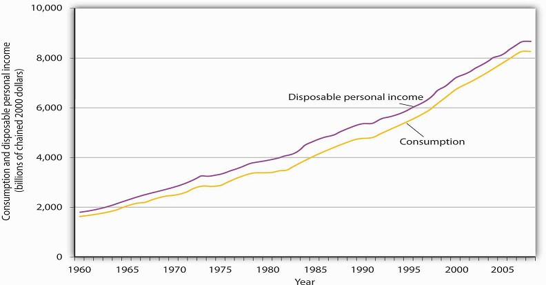
Source: U. S. Department of Commerce, Bureau of Economic Analysis, NIPA Tables 1.16 and 2.1 (December 23, 2008 revision; Data are through 3rd quarter 2008).
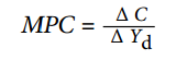
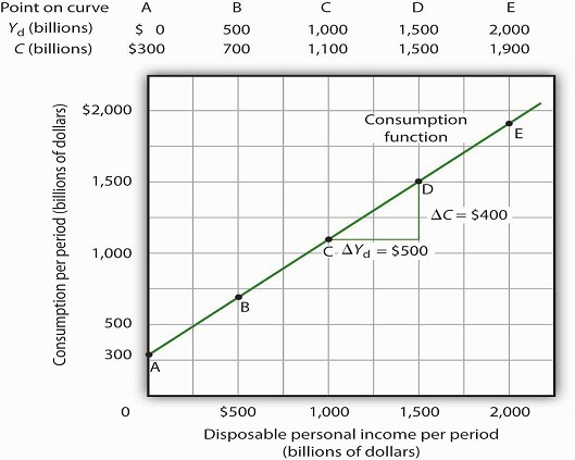
Figure 28.2 illustrates the consumption function. The relationship between consumption and disposable personal income that we encountered in Figure 28.1 is evident in the table and in the curve: consumption in any period increases as disposable personal income increases in that period. The slope of the consumption function tells us by how much. Consider points C and D. When disposable personal income (Yd) rises by $500 billion, consumption rises by $400 billion. More generally, the slope equals the change in consumption divided by the change in disposable personal income. The ratio of the change in consumption (ΔC) to the change in disposable personal income (ΔYd) is the marginal propensity to consume (MPC). The Greek letter delta (Δ) is used to denote “change in.”
EQUATION 28.1
In this case, the marginal propensity to consume equals $400/$500 = 0.8. It can be interpreted as the fraction of an extra $1 of disposable personal income that people spend on consumption. Thus, if a person with an MPC of 0.8 received an extra $1,000 of disposable personal income, that person’s consumption would rise by $0.80 for each extra $1 of disposable personal income, or $800.
We can also express the consumption function as an equation
EQUATION 28.2
C = $300 billion + 0.8Yd
Heads Up!
It is important to note carefully the definition of the marginal propensity to consume. It is the change in consumption divided by the change in disposable personal income. It is not the level of consumption divided by the level of disposable personal income. Using Equation 28.2, at a level of disposable personal income of $500 billion, for example, the level of consumption will be $700 billion so that the ratio of consumption to disposable personal income will be 1.4, while the marginal propensity to consume remains 0.8. The marginal propensity to consume is, as its name implies, a marginal concept. It tells us what will happen to an additional dollar of personal disposable income.
Notice from the curve in Figure 28.2 that when disposable personal income equals 0, consumption is $300 billion. The vertical intercept of the consumption function is thus $300 billion. Then, for every $500 billion increase in disposable personal income, consumption rises by $400 billion. Because the consumption function in our example is linear, its slope is the same between any two points. In this case, the slope of the consumption function, which is the same as the marginal propensity to consume, is 0.8 all along its length.
We can use the consumption function to show the relationship between personal saving and disposable personal income. Personal saving is disposable personal income not spent on consumption during a particular period; the value of personal saving for any period is found by subtracting consumption from disposable personal income for that period:
EQUATION 28.3
Personal saving = disposable personal income−consumption
The saving function relates personal saving in any period to disposable personal income in that period. Personal saving is not the only form of saving—firms and government agencies may save as well. In this chapter, however, our focus is on the choice households make between using disposable personal income for consumption or for personal saving.
Figure 28.3 shows how the consumption function and the saving function are related. Personal saving is calculated by subtracting values for consumption from values for disposable personal income, as shown in the table. The values for personal saving are then plotted in the graph. Notice that a 45 degree ine has been added to the graph. At every point on the 45-degree line, the value on the vertical axis equals that on the horizontal axis. The consumption function intersects the 45-degree line at an income of $1,500 billion (point D). At this point, consumption equals disposable personal income and personal saving equals 0 (point D’ on the graph of personal saving). Using the graph to find personal saving at other levels of disposable personal income, we subtract the value of consumption, given by the consumption function, from disposable personal income, given by the 45-degree line.
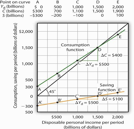
Personal saving equals disposable personal income minus consumption. The table gives hypothetical values for these variables. The consumption function is plotted in the upper part of the graph. At points along the 45-degree line, the values on the two axes are equal; we can measure personal saving as the distance between the 45-degree line and consumption. The curve of the saving function is in the lower portion of the graph.
At a disposable personal income of $2,000 billion, for example, consumption is $1,900 billion (point E).Personal saving equals $100 billion (point E')—the vertical distance between the 45-degree line and the consumption function. At an income of $500 billion, consumption totals $700 billion (point B). The consumption function lies above the 45-degree line at this point; personal saving is −$200 billion (point B'). A negative value for saving means that consumption exceeds disposable personal income; it must have come from saving accumulated in the past, from selling assets, or from borrowing.
Notice that for every $500 billion increase in disposable personal income, personal saving rises by $100 billion. Consider points C' and D' in Figure 28.3. When disposable personal income rises by $500 billion, personal saving rises by $100 billion. More generally, the slope of the saving function equals the change in personal saving divided by the change in disposable personal income. The ratio of the change in personal saving (ΔS) to the change in disposable personal income (ΔYd) is the marginal propensity to save (MPS).
EQUATION 28.4
In this case, the marginal propensity to save equals $100/$500 = 0.2. It can be interpreted as the fraction of an extra $1 of disposable personal income that people save. Thus, if a person with an MPS of 0.2 received an extra $1,000 of disposable personal income, that person’s saving would rise by $0.20 for each extra $1 of disposable personal income, or $200. Since people have only two choices of what to do with additional disposable personal income—that is, they can use it either for consumption or for personal saving—the fraction of disposable personal income that people consume (MPC) plus the fraction of disposable personal income that people save (MPS) must add to 1:
EQUATION 28.5
MPC + MPS = 1
- 10192 reads
