


The concept of the marginal propensity to consume suggests that consumption contains induced aggregate expenditures; an increase in real GDP raises consumption. But consumption contains an autonomous component as well. The level of consumption at the intersection of the consumption function and the vertical axis is regarded as autonomous consumption; this level of spending would occur regardless of the level of real GDP.
Consider the consumption function we used in deriving the schedule and curve illustrated in Figure 28.2
C = $300 billion+0.8Y
We can omit the subscript on disposable personal income because of the simplifications we have made in this section, and the symbol Y can be thought of as representing both disposable personal income and GDP. Because we assume that the price level in the aggregate expenditures model is constant, GDP equals real GDP. At every level of real GDP, consumption includes $300 billion in autonomous aggregate expenditures. It will also contain expenditures “induced” by the level of real GDP. At a level of real GDP of $2,000 billion, for example, consumption equals $1,900 billion: $300 billion in autonomous aggregate expenditures and $1,600 billion in consumption induced by the $2,000 billion level of real GDP.
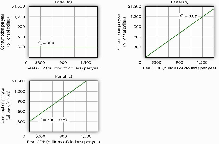
Figure 28.6 illustrates these two components of consumption. Autonomous consumption, Ca, which is always $300 billion, is shown in Panel (a); its equation is
EQUATION 28.7
Ca = $300 billion
Induced consumption Ci is shown in Panel (b); its equation is
EQUATION 28.8 Ci= 0.8Y
The consumption function is given by the sum of Equation 28.7 and Equation 28.8; it is shown in Panel (c) of Figure 28.5. It is the same as the equation C = $300 billion + 0.8Yd, since in this simple example, Y and Yd are the same.
Plotting the Aggregate Expenditures Curve
In this simplified economy, investment is the only other component of aggregate expenditures. We shall assume that investment is autonomous and that firms plan to invest $1,100 billion per year.
EQUATION 28.9 IP = $1,100 billion
The level of planned investment is unaffected by the level of real GDP.
Aggregate expenditures equal the sum of consumption C and planned investment IP. The aggregate expenditures function is the relationship of aggregate expenditures to the value of real GDP. It can be represented with an equation, as a table, or as a curve. We begin with the definition of aggregate expenditures AE when there is no government or foreign sector:
EQUATION 28.10
AE = C + IP
Substituting the information from above on consumption and planned investment yields (throughout this discussion all values are in billions of base-year dollars) AE = $300 + 0.8Y + $1,100
or
EQUATION 28.11 AE = $1,400 + 0.8Y
Equation 28.11 is the algebraic representation of the aggregate expenditures function. We shall use this equation to determine the equilibrium level of real GDP in the aggregate expenditures model. It is important to keep in mind that aggregate expenditures measure total planned spending at each level of real GDP (for any given price level). Real GDP is total production. Aggregate expenditures and real GDP need not be equal, and indeed will not be equal except when the economy is operating at its equilibrium level, as we will see in the next section.
In Equation 28.11, the autonomous component of aggregate expenditures is $1,400 billion, and the induced component is 0.8Y. We shall plot this aggregate expenditures function. To do so, we arbitrarily select various levels of real GDP and then use Equation 28.10 to compute aggregate expenditures at each level. At a level of real GDP of $6,000 billion, for example, aggregate expenditures equal $6,200 billion: AE = $1,400 + 0.8($6,000) = $6,200
The table in Figure 28.7 shows the values of aggregate expenditures at various levels of real GDP. Based on these values, we plot the aggregate expenditures curve. To obtain each value for aggregate expenditures, we simply insert the corresponding value for real GDP into Equation 28.11. The value at which the aggregate expenditures curve intersects the vertical axis corresponds to the level of autonomous aggregate expenditures. In our example, autonomous aggregate expenditures equal $1,400 billion. That figure includes $1,100 billion in planned investment, which is assumed to be autonomous, and $300 billion in autonomous consumption expenditure.
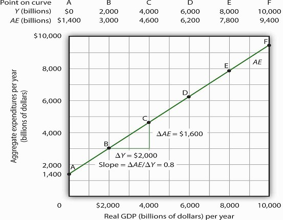
Values for aggregate expenditures AE are computed by inserting values for real GDP into Equation 28.10; these are given in the aggregate expenditures schedule. The point at which the aggregate expenditures curve intersects the vertical axis is the value of autonomous aggregate expenditures, here $1,400 billion. The slope of this aggregate expenditures curve is 0.8.
- 14131 reads
