


In the aggregate expenditures model, equilibrium is found at the level of real GDP at which the aggregate expenditures curve crosses the 45-degree line. It follows that a shift in the curve will change equilibrium real GDP. Here we will examine the magnitude of such changes.
Figure 28.10 begins with the aggregate expenditures curve shown in Figure 28.8. Now suppose that planned investment increases from the original value of $1,100 billion to a new value of $1,400 billion
— an increase of $300 billion. This increase in planned investment shifts the aggregate expenditures curve upward by $300 billion, all other things unchanged. Notice, however, that the new aggregate expenditures curve intersects the 45-degree line at a real GDP of $8,500 billion. The $300 billion increase in planned investment has produced an increase in equilibrium real GDP of $1,500 billion.
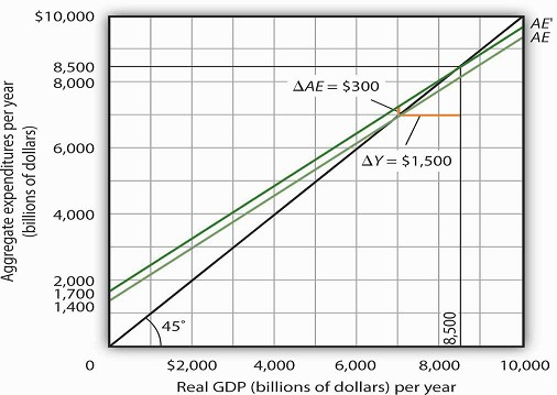
How could an increase in aggregate expenditures of $300 billion produce an increase in equilibrium real GDP of $1,500 billion? The answer lies in the operation of the multiplier. Because firms have increased their demand for investment goods (that is, for capital) by $300 billion, the firms that produce those goods will have $300 billion in additional orders. They will produce $300 billion in additional real GDP and, given our simplifying assumption, $300 billion in additional disposable personal income. But in this economy, each $1 of additional real GDP induces $0.80 in additional consumption. The $300 billion increase in autonomous aggregate expenditures initially induces $240 billion (= 0.8 × $300 billion) in additional consumption.
The $240 billion in additional consumption boosts production, creating another $240 billion in real GDP. But that second round of increase in real GDP induces $192 billion (= 0.8 × $240) in additional consumption, creating still more production, still more income, and still more consumption. Eventually (after many additional rounds of increases in induced consumption), the $300 billion increase in aggregate expenditures will result in a $1,500 billion increase in equilibrium real GDP. The following Table 28.1 shows the multiplied effect of a $300 billion increase in autonomous aggregate expenditures, assuming each $1 of additional real GDP induces $0.80 in additional consumption.
|
Round of spending |
Increase in real GDP (billions of dollars) |
|---|---|
|
1 |
$300 |
|
2 |
240 |
|
3 |
192 |
|
4 |
154 |
|
5 |
123 |
|
6 |
98 |
|
7 |
79 |
|
8 |
63 |
|
9 |
50 |
|
10 |
40 |
|
11 |
32 |
|
12 |
26 |
|
Subsequent rounds |
+103 |
|
Total increase in real GDP |
$1,500 |
A $300 billion increase in autonomous aggregate expenditures initially increases real GDP and income by that amount. This is shown in the first round of spending. The increased income leads to additional consumption. The additional consumption boosts production and thus leads to even higher real GDP and income. Assuming each $1 of additional real GDP induces $0.80 in additional consumption, the multiplied effect of a $300 billion increase in autonomous aggregate expenditures leads to additional rounds of spending such that, in this example, real GDP rises by $1,500 billion.
The size of the additional rounds of expenditure is based on the slope of the aggregate expenditures function, which in this example is simply the marginal propensity to consume. Had the slope been flatter (if the marginal propensity to consume were smaller), the additional rounds of spending would have been smaller. A steeper slope would mean that the additional rounds of spending would have been larger.
This process could also work in reverse. That is, a decrease in planned investment would lead to a multiplied decrease in real GDP. A reduction in planned investment would reduce the incomes of some households. They would reduce their consumption by the MPC times the reduction in their income. That, in turn, would reduce incomes for households that would have received the spending by the first group of households. The process continues, thus multiplying the impact of the reduction in aggregate expenditures resulting from the reduction in planned investment.
Computation of the Multiplier
The multiplier is the number by which we multiply an initial change in aggregate demand to get the full amount of the shift in the aggregate demand curve. Because the multiplier shows the amount by which the aggregate demand curve shifts at a given price level, and the aggregate expenditures model assumes a given price level, we can use the aggregate expenditures model to derive the multiplier explicitly.
Let Yeq be the equilibrium level of real GDP in the aggregate expenditures model, and let A be autonomous aggregate expenditures. Then the multiplier is
EQUATION 28.12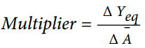
In the example we have just discussed, a change in autonomous aggregate expenditures of $300 billion produced a change in equilibrium real GDP of $1,500 billion. The value of the multiplier is therefore $1,500/$300 = 5.
The multiplier effect works because a change in autonomous aggregate expenditures causes a change in real GDP and disposable personal income, inducing a further change in the level of aggregate expenditures, which creates still more GDP and thus an even higher level of aggregate expenditures.The degree to which a given change in real GDP induces a change in aggregate expenditures is given in this simplified economy by the marginal propensity to consume, which, in this case, is the slope of the aggregate expenditures curve. The slope of the aggregate expenditures curve is thus linked to the size of the multiplier. We turn now to an investigation of the relationship between the marginal propensity to consume and the multiplier.
The Marginal Propensity to Consume and the Multiplier
We can compute the multiplier for this simplified economy from the marginal propensity to consume.
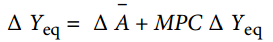
We know that the amount by which equilibrium real GDP will change as a result of a change in aggregate expenditures consists of two parts: the change in autonomous aggregate expenditures itself, Δ ¯A, and the induced change in spending. This induced change equals the marginal propensity to consume times the change in equilibrium real GDP, ΔYeq. Thus
EQUATION 28.13
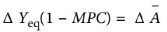
Subtract the MPCΔYeq term from both sides of the equation:
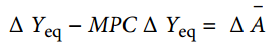
Factor out the ΔYeq term on the left:
Finally, solve for the multiplier 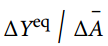 by dividing both
sides of the equation above by ΔA and by dividing both sides by (1 − MPC). We get the following:
by dividing both
sides of the equation above by ΔA and by dividing both sides by (1 − MPC). We get the following:
EQUATION 28.14
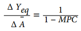
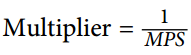
We thus compute the multiplier by taking 1 minus the marginal propensity to consume, then dividing the result into 1. In our example, the marginal propensity to consume is 0.8; the multiplier is 5, as we have already seen [multiplier = 1/(1 − MPC) = 1/(1 − 0.8) = 1/0.2 = 5]. Since the sum of the marginal propensity to consume and the marginal propensity to save is 1, the denominator on the right-hand side of Equation 28.13 is equivalent to the MPS, and the multiplier could also be expressed as 1/MPS.
EQUATION 28.15
We can rearrange terms in Equation 28.14 to use the multiplier to compute the impact of a change in autonomous aggregate expenditures. We simply multiply both sides of the equation by ¯A to obtain the following:
EQUATION 28.16
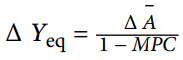
The change in the equilibrium level of income in the aggregate expenditures model (remember that the model assumes a constant price level) equals the change in autonomous aggregate expenditures times the multiplier. Thus, the greater the multiplier, the greater will be the impact on income of a change in autonomous aggregate expenditures.
- 5403 reads
