


Suppose that government purchases and net exports are autonomous. If so, they enter the aggregate expenditures function in the same way that investment did. Compared to the simplified aggregate expenditures model, the aggregate expenditures curve shifts up by the amount of government purchases and net exports.
Figure 28.11 shows the difference between the aggregate expenditures model of the simplified economy in Figure 28.8 and a more realistic view of the economy. Panel (a) shows an AE curve for an economy with only consumption and investment expenditures. In Panel (b), the AE curve includes all four components of aggregate expenditures.
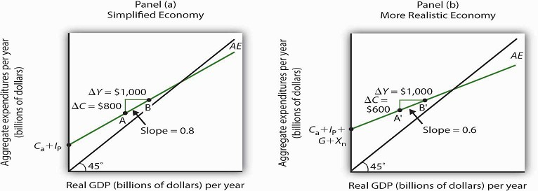
Panel (a) shows an aggregate expenditures curve for a simplified view of the economy; Panel (b) shows an aggregate expenditures curve for a more realistic model. The AE curve in Panel (b) has a higher intercept than the AE curve in Panel (a) because of the additional components of autonomous aggregate expenditures in a more realistic view of the economy. The slope of the AE curve in Panel (b) is flatter than the slope of the AE curve in Panel (a). In a simplified economy, the slope of the AE curve is the marginal propensity to consume (MPC). In a more realistic view of the economy, it is less than the MPC because of the difference between real GDP and disposable personal income.
There are two major differences between the aggregate expenditures curves shown in the two panels.Notice first that the intercept of the AE curve in Panel (b) is higher than that of the AE curve in Panel (a). The reason is that, in addition to the autonomous part of consumption and planned investment, there are two other components of aggregate expenditures—government purchases and net exports—that we have also assumed are autonomous. Thus, the intercept of the aggregate expenditures curve in Panel (b) is the sum of the four autonomous aggregate expenditures components: consumption (Ca), planned investment (IP), government purchases (G), and net exports (Xn). In Panel (a), the intercept includes only the first two components.
Second, notice that the slope of the aggregate expenditures curve is flatter for the more realistic economy in Panel (b) than it is for the simplified economy in Panel (a). This can be seen by comparing the slope of the aggregate expenditures curve between points A and B in Panel (a) to the slope of the aggregate expenditures curve between points A’ and B’ in Panel (b). Between both sets of points, real GDP changes by the same amount, $1,000 billion. In Panel (a), consumption rises by $800 billion, whereas in Panel (b) consumption rises by only $600 billion. This difference occurs because, in the more realistic view of the economy, households have only a fraction of real GDP available as disposable personal income. Thus, for a given change in real GDP, consumption rises by a smaller amount.
Let us examine what happens to equilibrium real GDP in each case if there is a shift in autonomous aggregate expenditures, such as an increase in planned investment, as shown in Figure 28.12. In both panels, the initial level of equilibrium real GDP is the same, Y1. Equilibrium real GDP occurs where the given aggregate expenditures curve intersects the 45-degree line. The aggregate expenditures curve shifts up by the same amount—ΔA is the same in both panels. The new level of equilibrium real GDP occurs where the new AE curve intersects the 45-degree line. In Panel (a), we see that the new level of equilibrium real GDP rises to Y2, but in Panel (b) it rises only to Y3. Since the same change in autonomous aggregate expenditures led to a greater increase in equilibrium real GDP in Panel (a) than in Panel (b), the multiplier for the more realistic model of the economy must be smaller. The multiplier is smaller, of course, because the slope of the aggregate expenditures curve is flatter.
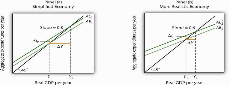
In Panels (a) and (b), equilibrium real GDP is initially Y1. Then autonomous aggregate expenditures rise by the same amount, ΔIP. In Panel (a), the upward shift in the AE curve leads to a new level of equilibrium real GDP of Y2; in Panel (b) equilibrium real GDP rises to Y3. Because equilibrium real GDP rises by more in Panel (a) than in Panel (b), the multiplier in the simplified economy is greater than in the more realistic one.
KEY TAKEAWAYS
- The aggregate expenditures model relates aggregate expenditures to real GDP. Equilibrium in the model occurs where aggregate expenditures equal real GDP and is found graphically at the intersection of the aggregate expenditures curve and the 45-degree line.
- Economists distinguish between autonomous and induced aggregate expenditures. The former do not vary with GDP; the latter do.
- Equilibrium in the aggregate expenditures model implies that unintended investment equals zero.
- A change in autonomous aggregate expenditures leads to a change in equilibrium real GDP, which is a multiple of the change in autonomous aggregate expenditures.
- The size of the multiplier depends on the slope of the aggregate expenditures curve. In general, the steeper the aggregate expenditures curve, the greater the multiplier. The flatter the aggregate expenditures curve, the smaller the multiplier.
- Income taxes tend to flatten the aggregate expenditures curve.
TRYIT!
Suppose you are given the following data for an economy. All data are in billions of dollars. Y is actual real GDP, and C, IP, G, and Xn are the consumption, planned investment, government purchases, and net exports components of aggregate expenditures, respectively.
| Y | C | IP | G | Xn |
|---|---|---|---|---|
| $0 | $800 | $1,000 | $1,400 | -$200 |
| 2,500 | 2,300 | 1,000 | 1,400 | -200 |
| 5,000 | 3,800 | 1,000 | 1,400 | -200 |
| 7,500 | 5,300 | 1,000 | 1,400 | -200 |
| 10,000 | 6,800 | 1,000 | 1,400 | -200 |
- Plot the corresponding aggregate expenditures curve and draw in the 45-degree line.
- What is the intercept of the AE curve? What is its slope?
- Determine the equilibrium level of real GDP.
- Now suppose that net exports fall by $1,000 billion and that this is the only change in autonomous aggregate expenditures. Plot the new aggregate expenditures curve. What is the new equilibrium level of real GDP?
- What is the value of the multiplier?
Case in Point: Fiscal Policy in the Kennedy Administration
It was the first time expansionary fiscal policy had ever been proposed. The economy had slipped into a recession in 1960. Presidential candidate John Kennedy received proposals from several
economists that year for a tax cut aimed at stimulating the economy. As a candidate, he was unconvinced. But, as president he proposed the tax cut in 1962. His chief economic adviser, Walter
Heller, defended the tax cut idea before Congress and introduced what was politically a novel concept: the multiplier.
In testimony to the Senate Subcommittee on Employment and Manpower, Mr. Heller predicted that a $10 billion cut in personal income taxes would boost consumption “by over $9 billion.”
To assess the ultimate impact of the tax cut, Mr. Heller applied the aggregate expenditures model. He rounded the increased consumption off to $9 billion and explained,
“This is far from the end of the matter. The higher production of consumer goods to meet this extra spending would mean extra employment, higher payrolls, higher profits, and higher farm and
professional and service incomes. This added purchasing power would generate still further increases in spending and incomes. … The initial rise of $9 billion, plus this extra consumption
spending and extra output of consumer goods, would add over $18 billion to our annual GDP.”
We can summarize this continuing process by saying that a “multiplier” of approximately 2 has been applied to the direct increment of consumption spending.
Mr. Heller also predicted that proposed cuts in corporate income tax rates would increase investment by about $6 billion. The total change in autonomous aggregate expenditures would thus be
$15 billion: $9 billion in consumption and $6 billion in investment. He predicted that the total increase in equilibrium GDP would be $30 billion, the amount the Council of Economic Advisers
had estimated would be necessary to reach full employment.
In the end, the tax cut was not passed until 1964, after President Kennedy’s assassination in 1963. While the Council of Economic Advisers concluded that the tax cut had worked as advertised,
it came long after the economy had recovered and tended to push the economy into an inflationary gap. As we will see in later chapters, the tax cut helped push the economy into a period of
rising inflation.
Source: Economic Report of the President 1964 (Washington, DC: U.S. Government Printing Office, 1964), 172–73.
ANSWERS TO TRYIT! PROBLEMS
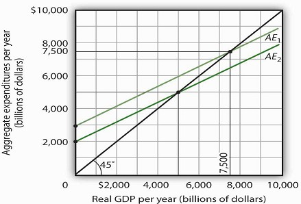
- The aggregate expenditures curve is plotted in the accompanying chart as AE1.
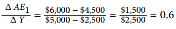
- The intercept of the AE1 curve is $3,000. It is the amount of aggregate expenditures (C + IP + G + Xn) when real GDP is zero. The slope of the AE1 curve is 0.6. It can be found by
determining the amount of aggregate expenditures for any two levels of real GDP and then by dividing the change in aggregate expenditures by the change in real GDP over the interval. For
example, between real GDP of $2,500 and $5,000, aggregate expenditures go from $4,500 to $6,000. Thus,
- The equilibrium level of real GDP is $7,500. It can be found by determining the intersection of AE1 and the 45-degree line. At Y = $7,500, AE1 = $5,300 + 1,000 + 1,400 − 200 = $7,500.
- A reduction of net exports of $1,000 shifts the aggregate expenditures curve down by $1,000 to AE2. The equilibrium real GDP falls from $7,500 to $5,000. The new aggregate expenditures curve, AE2, intersects the 45-degree line at real GDP of $5,000.
- The multiplier is 2.5 [= (−$2,500)/(−$1,000)].
- 3794 reads
