


An aggregate expenditures curve assumes a fixed price level. If the price level were to change, the levels of consumption, investment, and net exports would all change, producing a new aggregate expenditures curve and a new equilibrium solution in the aggregate expenditures model.
A change in the price level changes people’s real wealth. Suppose, for example, that your wealth includes $10,000 in a bond account. An increase in the price level would reduce the real value of this money, reduce your real wealth, and thus reduce your consumption. Similarly, a reduction in the price level would increase the real value of money holdings and thus increase real wealth and consumption. The tendency for price level changes to change real wealth and consumption is called the wealth effect.
Because changes in the price level also affect the real quantity of money, we can expect a change in the price level to change the interest rate. A reduction in the price level will increase the real quantity of money and thus lower the interest rate. A lower interest rate, all other things unchanged, will increase the level of investment. Similarly, a higher price level reduces the real quantity of money, raises interest rates, and reduces investment. This is called the interest rate effect.
Finally, a change in the domestic price level will affect exports and imports. A higher price level makes a country’s exports fall and imports rise, reducing net exports. A lower price level will increase exports and reduce imports, increasing net exports. This impact of different price levels on the level of net exports is called the international trade effect.
Panel (a) of Figure 28.13 shows three possible aggregate expenditures curves for three different price levels. For example, the aggregate expenditures curve labeled AEP=1.0 is the aggregate expenditures curve for an economy with a price level of 1.0. Since that aggregate expenditures curve crosses the 45-degree line at $6,000 billion, equilibrium real GDP is $6,000 billion at that price level. At a lower price level, aggregate expenditures would rise because of the wealth effect, the interest rate effect, and the international trade effect. Assume that at every level of real GDP, a reduction in the price level to 0.5 would boost aggregate expenditures by $2,000 billion to AEP = 0.5, and an increase in the price level from 1.0 to 1.5 would reduce aggregate expenditures by $2,000 billion. The aggregate expenditures curve for a price level of 1.5 is shown as AEP=1.5. There is a different aggregate expenditures curve, and
a different level of equilibrium real GDP, for each of these three price levels. A price level of 1.5 produces equilibrium at point A, a price level of 1.0 does so at point B, and a price level of 0.5 does so at point C. More generally, there will be a different level of equilibrium real GDP for every price level; the higher the price level, the lower the equilibrium value of real GDP.
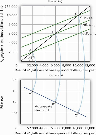
Because there is a different aggregate expenditures curve for each price level, there is a different equilibrium real GDP for each price level. Panel (a) shows aggregate expenditures curves for three different price levels. Panel (b)shows that the aggregate demand curve, which shows the quantity of goods and services demanded at each price level, can thus be derived from the aggregate expenditures model. The aggregate expenditures curve for a price level of 1.0, for example, intersects the 45-degree line in Panel (a) at point B, producing an equilibrium real GDP of $6,000 billion. We can thus plot point B′ on the aggregate demand curve in Panel (b), which shows that at a price level of 1.0, a real GDP of $6,000 billion is demanded.
Panel (b) of Figure 28.13 shows how an aggregate demand curve can be derived from the aggregate expenditures curves for different price levels. The equilibrium real GDP associated with each price level in the aggregate expenditures model is plotted as a point showing the price level and the quantity of goods and services demanded (measured as real GDP). At a price level of 1.0, for example, the equilibrium level of real GDP in the aggregate expenditures model in Panel (a) is $6,000 billion at point B. That means $6,000 billion worth of goods and services is demanded; point B’ on the aggregate demand curve in Panel (b) corresponds to a real GDP demanded of $6,000 billion and a price level of 1.0. At a price level of 0.5 the equilibrium GDP demanded is $10,000 billion at point C’, and at a price level of 1.5 the equilibrium real GDP demanded is $2,000 billion at point A’. The aggregate demand curve thus shows the equilibrium real GDP from the aggregate expenditures model at each price level.
- 5864 reads
