


The ratio of the output and input amplitudes for Figure 3.29 ,known as the transfer function or the frequency response, is given by
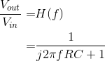
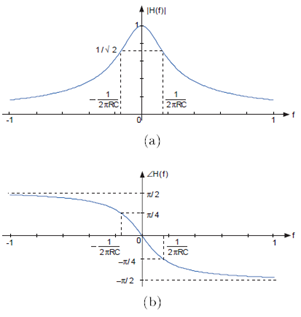
Implicit in using the transfer function is that the input is a complex exponential, and the output is also a complex exponential having the same frequency. The transfer function reveals how the circuit modifies the input amplitude in creating the output amplitude. Thus, the transfer function completely describes how the circuit processes the input complex exponential to produce the output complex exponential. The circuit's function is thus summarized by the transfer function. In fact, circuits are often designed to meet transfer function specifications. Because transfer functions are complex-valued, frequency-dependent quantities, we can better appreciate a circuit's function by examining the magnitude and phase of its transfer function (Figure 3.30 (Magnitude and phase of the transfer function)).
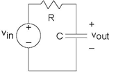
Simple Circuit
(a) 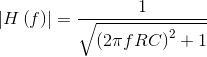 (b)
(b)
This transfer function has many important properties and provides all the insights needed to determine how the circuit functions. First of all, note that we can
compute the frequency response for both positive and negative frequencies. Recall that sinusoids consist of the sum of two complex exponentials, one having the negative frequency of the other.
We will consider how the circuit acts on a sinusoid soon. Do note that the magnitude has even symmetry: The negative frequency portion is a mirror image of the
positive frequency portion: |H (−f) | = |H (f) |. The phase has odd symmetry: ∠ (H (−f)) = −(∠ (H
(f)). These properties of this specific example apply for all transfer functions associated with circuits. Consequently, we don't need to plot the
negative frequency component; we know what it is from the positive frequency part. The magnitude equals  of its maximum gain (1 at f =0) when 2πfRC =1 (the two terms in the 2 denominator of the magnitude are
equal). The frequency
of its maximum gain (1 at f =0) when 2πfRC =1 (the two terms in the 2 denominator of the magnitude are
equal). The frequency  defines the boundary between two operating
ranges.
defines the boundary between two operating
ranges.
- For frequencies below this frequency, the circuit does not much alter the amplitude of the complex exponential source.
- For frequencies greater than fc, the circuit strongly attenuates the amplitude. Thus, when the source frequency is in this range, the circuit's output has a much smaller amplitude than that of the source.
For these reasons, this frequency is known as the cutoff frequency. In this circuit the cutoff
frequency depends only on the product of the resistance and the capacitance. Thus, a cutoff frequency of 1 kHz occurs when  or
or 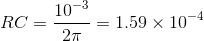 . Thus resistance-capacitance combinations of 1.59 kΩ and 100nF or 10 Ω and 1.59 µF result in the same
cutoff frequency.
. Thus resistance-capacitance combinations of 1.59 kΩ and 100nF or 10 Ω and 1.59 µF result in the same
cutoff frequency.
The phase shift caused by the circuit at the cutoff frequency precisely equals  Thus, below the cutoff frequency, phase is little affected, but at higher frequencies, the phase shift caused by the circuit becomes
 This phase shift corresponds to the difference between
a cosine and a sine.
This phase shift corresponds to the difference between
a cosine and a sine.
We can use the transfer function to find the output when the input voltage is a sinusoid for two reasons. First of all, a sinusoid is the sum of two complex exponentials, each having a frequency equal to the negative of the other. Secondly, because the circuit is linear, superposition applies. If the source is a sine wave, we know that
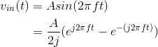
Since the input is the sum of two complex exponentials, we know that the output is also a sum of two similar complex exponentials, the only difference being that the complex amplitude of each is multiplied by the transfer function evaluated at each exponential's frequency.
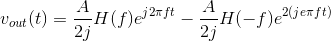
As noted earlier, the transfer function is most conveniently expressed in polar form: H (f)=|H (f) |e j∠(H(f). Furthermore, |H (−f) | = |H (f) | (even symmetry of the magnitude) and ∠ (H (−f)) = −(∠ (H (f)) (odd symmetry of the phase). The output voltage expression simplifes to
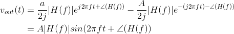
The circuit's output to a sinusoidal input is also a sinusoid, having a gain equal to the magnitude of the circuit's transfer function evaluated at the source frequency and a phase equal to the phase of the transfer function at the source frequency. It will turn out that this input-output relation description applies to any linear circuit having a sinusoidal source.
Exercise 3.13.1
This input-output property is a special case of a more general result. Show that if the source can be written as the imaginary part of a complex exponential vin (t) = Im (Vej2πft) the output is given byvout (t) = Im(VH (f) e j2πft). Show that a similar result also holds for the real part.
The notion of impedance arises when we assume the sources are complex exponentials. This assumption may seem restrictive; what would we do if the source were a unit step? When we use impedances to find the transfer function between the source and the output variable, we can derive from it the differential equation that relates input and output. The differential equation applies no matter what the source may be. As we have argued, it is far simpler to use impedances to find the differential equation (because we can use series and parallel combination rules) than any other method. In this sense, we have not lost anything by temporarily pretending the source is a complex exponential.
In fact we can also solve the differential equation using impedances! Thus, despite the apparent restrictiveness of impedances, assuming complex exponential sources is actually quite general.
- 4931 reads
