Formal Circuit Methods: Node Method

Available under Creative Commons-ShareAlike 4.0 International License.

In some (complicated) cases, we cannot use the simplification techniques such as parallel or series combination rules to solve for a circuit's input-output relation. In other modules, we wrote v-i relations and Kirchhoff’s laws haphazardly, solving them more on intuition than procedure. We need a formal method that produces a small, easy set of equations that lead directly to the input-output relation we seek. One such technique is the node method.

Figure 3.33 Node Voltage

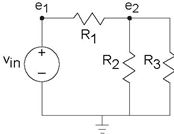
The node method begins by finding all nodes places where circuit elements attach to each other in the circuit. We call one of the nodes the reference node; the choice of reference node is arbitrary, but it is usually chosen to be a point of symmetry or the "bottom" node. For the remaining nodes, we define node voltages en that represent the voltage between the node and the reference. These node voltages constitute the only unknowns; all we need is a sufficient number of equations to solve for them. In our example, we have two node voltages. The very act of defining node voltages is equivalent to using all the KVL equations at your disposal. The reason for this simple, but astounding, fact is that a node voltage is uniquely defined regardless of what path is traced between the node and the reference. Because two paths between a node and reference have the same voltage, the sum of voltages around the loop equals zero.

In some cases, a node voltage corresponds exactly to the voltage across a voltage source. In such cases, the node voltage is specifed by the source and is not an unknown. For example, in our circuit, e1 = vin; thus, we need only to find one node voltage.

The equations governing the node voltages are obtained by writing KCL equations at each node having an unknown node voltage, using the v-i relations for each element. In our example, the only circuit equation is

$\frac{e_2-v_{in}}{R_1}+\frac{e_2}{R_2}+\frac{e_2}{R_3}=0$

A little refection reveals that when writing the KCL equations for the sum of currents leaving a node, that node's voltage will always appear with a plus sign, and all other node voltages with a minus sign. Systematic application of this procedure makes it easy to write node equations and to check them before solving them. Also remember to check units at this point: Every term should have units of current. In our example, solving for the unknown node voltage is easy:

$e_2=\frac{R_2R_3}{R_1R_2+R_1R_3+R_2R_3}v_{in}$

Have we really solved the circuit with the node method? Along the way, we have used KVL, KCL, and the v-i relations. Previously, we indicated that the set of equations resulting from applying these laws is necessary and sufficient. This result guarantees that the node method can be used to "solve" any circuit. One fallout of this result is that we must be able to find any circuit variable given the node voltages and sources. All circuit variables can be found using the v-i relations and voltage divider. For example, the current through R3 equals $\frac{e_2}{R_3}$ .

Figure 3.34 circuit example

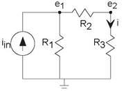
The presence of a current source in the circuit does not afect the node method greatly; just include it in writing KCL equations as a current leaving the node. The circuit has three nodes, requiring us to define two node voltages. The node equations are

$\frac{e_1}{R_1}+\frac{e_1-e_2}{R_2}-i_{in}=0$ (Node 1)
$\frac{e_2-e_1}{R_2}+\frac{e_2}{R_3}=0$
(Node 2)

Note that the node voltage corresponding to the node that we are writing KCL for enters with a positive sign, the others with a negative sign, and that the units of each term is given in amperes. Rewrite these equations in the standard set-of-linear-equations form.

$e_1\left ( \frac{1}{R_1}+\frac{1}{R_2} \right )-e_2\frac{1}{R_2}=i_{in}$
$(e_1)\frac{1}{R_2}+e_2\left ( \frac{1}{R_2}+\frac{1}{R_3} \right )=0$

Solving these equations gives

$e_1=\frac{R_2+R_3}{R_3}e_2$
$e_2=\frac{R_1R_3}{R_1+R_2+R_3}i_in$

To find the indicated current, we simply use $i=\frac{e_2}{R_3}$ .

Example 3.6: Node Method Example

Figure 3.35 circuit example 2

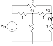
In this circuit (Figure 3.35), we cannot use the series/parallel combination rules: The vertical resistor at node 1 keeps the two horizontal 1 Ω resistors from being in series, and the 2 Ω resistor prevents the two 1 Ω resistors at node 2 from being in series. We really do need the node method to solve this circuit! Despite having six elements, we need only define two node voltages. The node equations are

$\frac{e_1-v_{in}}{1}+\frac{e_1}{1}+\frac{e_1-e_2}{1}=0$ (Node 1)
$\frac{e_2-v_{in}}{2}+\frac{e_2}{1}+\frac{e_2-e_1}{1}=0$
(Node 2)

Solving these equations yields $e_1=\frac{2}{5}v_{in}$ and $e_2=\frac{5}{13}v_{in}$ . The output current equals $\frac{e_2}{1}=\frac{5}{13}v_{in}.$
One unfortunate consequence of using the element's numeric values from the outset is that it becomes impossible to check units while setting up and solving equations.

Exercise 3.15.1

What is the equivalent resistance seen by the voltage source?

Figure 3.36 Node Method and Impedances

Modification of the circuit shown on the left to illustrate the node method and the effect of adding the resistor R2_.

The node method applies to RLC circuits, without significant modification from the methods used on simple resistive circuits, if we use complex amplitudes. We rely on the fact that complex amplitudes satisfy KVL, KCL, and impedance-based v-i relations. In the example circuit, we define complex amplitudes for the input and output variables and for the node voltages. We need only one node voltage here, and its KCL equation is
$\frac{E-V_{in}}{R_1}+Ej2\pi fC+\frac{E}{R_2}=0$
with the result
$E=\frac{R_2}{R_1+R_2+j2\pi fR_1R_2C}V_{in}$
To find the transfer function between input and output voltages, we compute the ratio $\frac{E}{V_{in}}$ . The transfer function's magnitude and angle are

To find the transfer function between input and output voltages, we compute the ratio media/image245.png . The transfer function's magnitude and angle are

$\left | H\left ( f \right ) \right |=\frac{R_{2}}{\sqrt{\left ( R_{1}+R_{2} \right )^{2}+\left (2\pi fR_{1}R_{2}C \right )^{2}}}$
$\angle (H(f))=-\left ( arctan\left ( \frac{2\pi f R_1R_2C}{R_1+R_2} \right ) \right )$

This circuit differs from the one shown previously (Figure 3.29: Simple Circuit) in that the resistor R₂ has been added across the output. What effect has it had on the transfer function, which in the original circuit was a lowpass filter having cutoff frequency $f_c=\frac{1}{2\pi R_1C}?$ As shown in Figure 3.37, adding the second resistor has two effects: it lowers the gain in the passband (the range of frequencies for which the filter has little effect on the input) and increases the cutoff frequency.

Figure 3.37 Transfer Function

Transfer functions of the circuits shown in Figure 3.36 (Node Method and Impedances). Here, R₁ =1, R₂ =1, and C = 1.

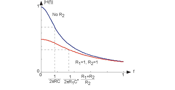
When R₂ = R₁, as shown on the plot, the passband gain becomes half of the original, and the cutoff frequency increases by the same factor. Thus, adding R₂ provides a 'knob' by which we can trade passband gain for cutoff frequency.

Exercise 3.15.2

We can change the cutoff frequency without affecting passband gain by changing the resistance in the original circuit. Does the addition of the R₂ resistor help in circuit design?

3050 reads

You are here

Formal Circuit Methods: Node Method