


In an earlier module (Exercise 2.3.1), we showed that a square wave could be expressed as a superposition of pulses. As useful as this decomposition was in this example, it does not generalize well to other periodic signals: How can a superposition of pulses equal a smooth signal like a sinusoid? Because of the importance of sinusoids to linear systems, you might wonder whether they could be added together to represent a large number of periodic signals. You would be right and in good company as well. Euler and Gauss in particular worried about this problem, and Jean Baptiste Fourier5 got the credit even though tough mathematical issues were not settled until later. They worked on what is now known as the Fourier series: representing any periodic signal as a superposition of sinusoids.
But the Fourier series goes well beyond being another signal decomposition method. Rather, the Fourier series begins our journey to appreciate how a signal can be described in either the
time-domain or the frequency-domain with no compromise. Let s (t) be a periodic signal with period
T. We want to show that periodic signals, even those that have constant-valued segments like a square wave, can be expressed as sum of harmonically related sine waves: sinusoids having frequencies that are integer multiples of the fundamental frequency. Because the signal has
period T , the fundamental frequency is  . The complex Fourier series
expresses the signal as a superposition of complex exponentials having frequencies
. The complex Fourier series
expresses the signal as a superposition of complex exponentials having frequencies  ,
,
k = {. . ., −1, 0, 1,...}.
with  The real and
imaginary parts of the Fourier coefficients ck are written in this unusual way for convenience
in defining the classic Fourier series. The zeroth coefficient equals the signal's average value and is real-valued for real-valued signals: c0
= a0. The family of functions
The real and
imaginary parts of the Fourier coefficients ck are written in this unusual way for convenience
in defining the classic Fourier series. The zeroth coefficient equals the signal's average value and is real-valued for real-valued signals: c0
= a0. The family of functions  are called basis functions and form the foundation of the Fourier series. No matter what the periodic
signal might be, these functions are always present and form the representation's building blocks. They depend on the signal period T, and are indexed by
k.
are called basis functions and form the foundation of the Fourier series. No matter what the periodic
signal might be, these functions are always present and form the representation's building blocks. They depend on the signal period T, and are indexed by
k.
KEY POINT: Assuming we know the period, knowing the Fourier coefficients is equivalent to knowing the signal. Thus, it makes no difference if we have a time-domain or a frequency-domain characterization of the signal.
Exercise 4.2.1
What is the complex Fourier series for a sinusoid? To find the Fourier coefficients, we note the orthogonality property
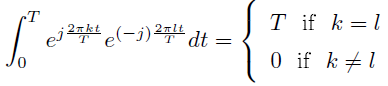
Assuming for the moment that the complex Fourier series "works," we can find a signal's complex Fourier coefficients, its spectrum, by exploiting the orthogonality properties of harmonically related complex exponentials. Simply multiply each side of (4.1) by e−(j2πlt) and integrate over the interval [0,T ].
Example 4.1
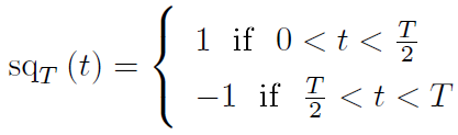
Finding the Fourier series coefficients for the square wave sqT(t) is very
simple. Mathematically, this signal can be expressed as
The expression for the Fourier coefficients has the form
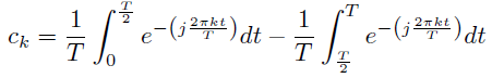
The two integrals are very similar, one equaling the negative of the other. The fnal expression becomes
Thus, the complex Fourier series for the square wave is
Consequently, the square wave equals a sum of complex exponentials, but only those having frequencies equal to odd multiples of the fundamental frequency  . The coefficients decay slowly as the frequency index k increases.
This index corresponds to the k-th harmonic of the signal's period.
. The coefficients decay slowly as the frequency index k increases.
This index corresponds to the k-th harmonic of the signal's period.
A signal's Fourier series spectrum ck has interesting properties.
Property 4.1:
If s (t) is real, ck = c−k* (real-valued periodic signals have conjugate-symmetric spectra). This result follows from the integral that calculates the ck from the signal. Furthermore, this result means that Re (ck)= Re (c−k): The real part of the Fourier coefficients for real-valued signals is even. Similarly, Im (ck)= −Im (c−k): The imaginary parts of the Fourier coefficients have odd symmetry. Consequently, if you are given the Fourier coefficients for positive indices and zero and are told the signal is real-valued, you can find the negative-indexed coefficients, hence the entire spectrum. This kind of symmetry, ck = c−k*, is known as conjugate symmetry.
Property 4.2:
If s (−t)= s (t), which says the signal has even symmetry about the origin, c−k = ck. Given the previous property for real-valued signals, the Fourier coefficients of even signals are real-valued. A real-valued Fourier expansion amounts to an expansion in terms of only cosines, which is the simplest example of an even signal.
Property 4.3:
If s(−t)= −(s(t)), which says the signal has odd symmetry, c−k = −ck. Therefore, the Fourier coefficients are purely imaginary. The square wave is a great example of an odd-symmetric signal.
Property 4.4:
The spectral coefficients for a periodic signal delayed by τ, s (t − τ), are  , where ck denotes the spectrum of
s(t). Delaying a signal by τ seconds results in a spectrum having a linear
phaseshift of
, where ck denotes the spectrum of
s(t). Delaying a signal by τ seconds results in a spectrum having a linear
phaseshift of  in comparison to the spectrum of the undelayed signal. Note that the spectral magnitude is unaffected. Showing this property is
easy.
in comparison to the spectrum of the undelayed signal. Note that the spectral magnitude is unaffected. Showing this property is
easy.
Proof:
Note that the range of integration extends over a period of the integrand. Consequently, it should not matter how we integrate over a period, which means that  , and we have our result.
The complex Fourier series obeys Parseval's Theorem, one of the most important results in signal analysis. This general mathematical result says you can calculate a signal's power in either the time domain or the frequency domain.
Theorem 4.1: Parseval's Theorem
Average power calculated in the time domain equals the power calculated in the frequency domain.
This result is a (simpler) re-expression of how to calculate a signal's power than with the real-valued Fourier series expression for power. Let's calculate the Fourier coefficients of the periodic pulse signal shown here (Figure 4.1).
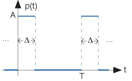
The pulse width is Δ, the period T , and the amplitude A. The complex Fourier spectrum of this signal is given by
At this point, simplifying this expression requires knowing an interesting property.
Armed with this result, we can simply express the Fourier series coefficients for our pulse sequence.
Because this signal is real-valued, we find that the coefficients do indeed have conjugate symmetry: ck= c−k * . The periodic pulse signal has neither even nor odd symmetry; consequently, no additional symmetry exists in the spectrum. Because the spectrum is complex valued, to plot it we need to calculate its magnitude and phase.
The function neg (·) equals -1 if its argument is negative and zero otherwise. The somewhat complicated expression for the phase results because the sine term can be negative; magnitudes must be positive, leaving the occasional negative values to be accounted for as a phase shift of π.
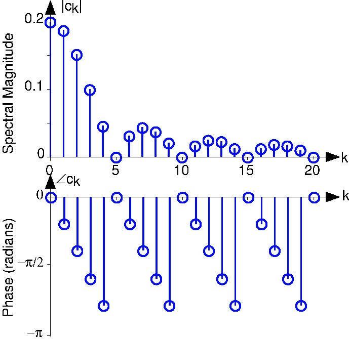
Also note the presence of a linear phase term (the first term in ∠ (ck) is proportional to frequency  ). Comparing this term with that predicted from delaying a signal, a delay of
  is present in our signal. Advancing the signal by this amount centers the
pulse about the origin, leaving an even signal, which in turn means that its spectrum is real-valued. Thus, our calculated spectrum is consistent with the properties of the Fourier spectrum.
is present in our signal. Advancing the signal by this amount centers the
pulse about the origin, leaving an even signal, which in turn means that its spectrum is real-valued. Thus, our calculated spectrum is consistent with the properties of the Fourier spectrum.
Exercise 4.2.2
What is the value of c0? Recalling that this spectral coefficient corresponds to the signal's average value, does your answer make sense?
The phase plot shown in Figure 4.2 requires some explanation as it does not seem to agree with what (4.10) suggests. There, the phase has a linear component, with a jump of π every time the sinusoidal term changes sign. We must realize that any integer multiple of 2π can be added to a phase at each frequency without affecting the value of the complex spectrum. We see that at frequency index 4 the phase is nearly −π. The phase at index 5 is undefined because the magnitude is zero in this example. At index 6, the formula suggests that the phase of the linear term should be less than −π (more negative). In addition, we expect a shift of −π in the phase between indices 4 and 6. Thus, the phase value predicted by the formula is a little less than − (2π). Because we can add 2π without affecting the value of the spectrum at index 6, the result is a slightly negative number as shown. Thus, the formula and the plot do agree. In phase calculations like those made in MATLAB, values are usually confined to the range [−π, π) by adding some (possibly negative) multiple of 2π to each phase value.
- 7374 reads
