


The discrete-time Fourier transform (and the continuous-time transform as well) can be evaluated when we have an analytic expression for the signal. Suppose we just have a signal, such as the speech signal used in the previous chapter, for which there is no formula. How then would you compute the spectrum? For example, how did we compute a spectrogram such as the one shown in the speech signal example (Figure 4.17: spectrogram)? The Discrete Fourier Transform (DFT) allows the computation of spectra from discrete-time data. While in discrete-time we can exactly calculate spectra, for analog signals no similar exact spectrum computation exists. For analog-signal spectra, use must build special devices, which turn out in most cases to consist of A/D converters and discrete-time computations. Certainly discrete-time spectral analysis is more flexible than continuous-time spectral analysis.
The formula for the DTFT (5.17) is a sum, which conceptually can be easily computed save for two issues.
- Signal duration. The sum extends over the signal's duration, which must be fnite to compute the signal's spectrum. It is exceedingly difcult to store an infnite-length signal in any case, so we'll assume that the signal extends over [0,N − 1].
-
Continuous frequency. Subtler than the signal duration issue is the fact that the frequency variable is continuous: It may only need to span one period, like
![\left [ -\left ( \frac{1}{2} \right ),\frac{1}{2} \right ]](/system/files/resource/9/9648/9756/media/eqn-img_31.gif) or [0, 1], but the
DTFT formula as it stands requires evaluating the spectra at all frequencies within a period. Let's compute the spectrum at a few frequencies; the most obvious ones are the equally
spaced ones
or [0, 1], but the
DTFT formula as it stands requires evaluating the spectra at all frequencies within a period. Let's compute the spectrum at a few frequencies; the most obvious ones are the equally
spaced ones 
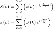
We thus define the discrete Fourier transform (DFT) to be
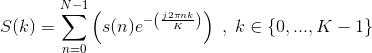
Here, S(k) is shorthand for 
We can compute the spectrum at as many equally spaced frequencies as we like. Note that you can think about this computationally motivated choice as sampling the
spectrum; more about this interpretation later. The issue now is how many frequencies are enough to capture how the spectrum changes with frequency. One way of answering this question is
determining an inverse discrete Fourier transform formula: given S(k), k = {0,...,K − 1} how do we find s(n), n = {0,...,N − 1}? Presumably, the formula will be of
the form 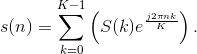 Substituting the DFT formula in this prototype inverse transform yields
Note that the orthogonality relation we use so often has a different character now.
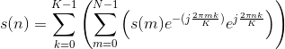
We obtain nonzero value whenever the two indices difer by multiples of K. We can express this result as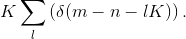 Thus, our formula becomes
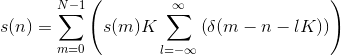
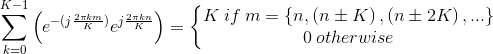
The integers n and m both range over {0,...,N − 1}. To have an inverse transform, we need the sum to be a single unit sample for m, n in this range. If it did not, then s (n) would equal a sum of values, and we would not have a valid transform: Once going into the frequency domain, we could not get back unambiguously! Clearly, the term l =0 always provides a unit sample (we'll take care of the factor of K soon). If we evaluate the spectrum at fewer frequencies than the signal's duration, the term corresponding to m = n + K will also appear for some values of m, n = {0,...,N - 1}. This situation means that our prototype transform equals s (n) + s (n + K) for some values of n. The only way to eliminate this problem is to require K ≥ N: We must have at least as many frequency samples as the signal's duration. In this way, we can return from the frequency domain we entered via the DFT.
Exercise 5.7.1
When we have fewer frequency samples than the signal's duration, some discrete-time signal values equal the sum of the original signal values. Given the sampling interpretation of the spectrum, characterize this effect a different way.
Another way to understand this requirement is to use the theory of linear equations. If we write out the expression for the DFT as a set of linear equations,


.....

we have K equations in N unknowns if we want to find the signal from its sampled spectrum. This require ment is impossible to fulfll if K < N; we must have K ≥ N. Our orthogonality relation essentially says that if we have a sufcient number of equations (frequency samples), the resulting set of equations can indeed be solved.
By convention, the number of DFT frequency values K is chosen to equal the signal's duration N. The discrete Fourier transform pair consists of
Discrete Fourier Transform Pair
Example 5.3
Use this demonstration to perform DFT analysis of a signal.
This media object is a LabVIEW VI. Please view or download it at
<DFTanalysis.llb>
Example 5.4
Use this demonstration to synthesize a signal from a DFT sequence.
This media object is a LabVIEW VI. Please view or download it at
<DFT_Component_Manipulation.llb>
- 2898 reads
