Efficiency of Frequency-Domain Filtering

Available under Creative Commons-ShareAlike 4.0 International License.

To determine for what signal and filter durations a time-or frequency-domain implementation would be the most efficient, we need only count the computations required by each. For the time-domain, difference equation approach, we need N_x (2 (q) + 1). The frequency-domain approach requires three Fourier transforms, each requiring $\left ( \frac{K}{2} \right )\left ( \log_{2}K \right )$ computations for a length-K FFT, and the multiplication of two spectra (6K computations). The output-signal-duration-determined length must be at least N_x + q. Thus, we must compare

$\left ( N_{x}\left ( 2q+1 \right )\leftrightarrow 6\left ( N_{x}+q \right )+\frac{3}{2}\left ( N_{x}+q \right )log_{2}\left ( N_{x}+q \right ) \right )$

Exact analytic evaluation of this comparison is quite difficult (we have a transcendental equation to solve). Insight into this comparison is best obtained by dividing by N_x.

$\left ( 2q+1\leftrightarrow 6 \left ( 1+\frac{q}{N_{x}} \right )+\frac{3}{2}\left ( 1+\frac{q}{N_{x}} \right )log_{2}\left ( N_{x}+q \right ) \right )$

With this manipulation, we are evaluating the number of computations per sample. For any given value of the filter's order q, the right side, the number of frequency-domain computations, will exceed the left if the signal's duration is long enough. However, for filter durations greater than about 10, as long as the input is at least 10 samples, the frequency-domain approach is faster so long as the FFT's power-of-two constraint is advantageous.

The frequency-domain approach is not yet viable; what will we do when the input signal is infinitely long? The difference equation scenario fits perfectly with the envisioned digital filtering structure (Figure 5.24), but so far we have required the input to have limited duration (so that we could calculate its Fourier transform). The solution to this problem is quite simple: Section the input into frames, filter each, and add the results together. To section a signal means expressing it as a linear combination of length-N_x non-overlapping "chunks." Because the filter is linear, filtering a sum of terms is equivalent to summing the results of filtering each term.

$x(n)=\sum_{m=-\infty }^{\infty }\left ( x\left ( n-mN_{x} \right ) \right ) \Rightarrow y(n) = \sum_{m=-\infty }^{\infty } \left ( y(n-mN_{x}) \right )$

(5.55)

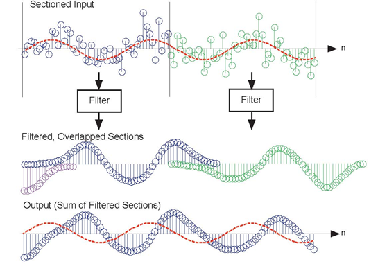
As illustrated in Figure 5.22, note that each filtered section has a duration longer than the input. Conse quently, we must literally add the filtered sections together, not just butt them together.

Figure 5.22

The noisy input signal is sectioned into length-48 frames, each of which is filtered using frequency-domain techniques. Each filtered section is added to other outputs that overlap to create the signal equivalent to having filtered the entire input. The sinusoidal component of the signal is shown as the red dashed line.

Computational considerations reveal a substantial advantage for a frequency-domain implementation over a time-domain one. The number of computations for a time-domain implementation essentially remains constant whether we section the input or not. Thus, the number of computations for each output is 2(q)+1. In the frequency-domain approach, computation counting changes because we need only compute the filter's frequency response H (k) once, which amounts to a fixed overhead. We need only compute two DFTs and multiply them to filter a section. Letting N_x denote a section's length, the number of computations for a section amounts to $(N_{x}+q)\log_{2}(N_{x}+q)+6(N_{x}+q).$ In addition, we must add the filtered outputs together; the number of terms to add corresponds to the excess duration of the output compared with the input (q). The frequency-domain approach thus requires $\left ( 1+\frac{q}{N_{x}} \right )\log_{2}\left ( N_{x}+q \right )+7\frac{q}{N_{x}}+6$ computations per output value. For even modest filter orders, the frequency-domain approach is much faster.

Exercise 5.15.1

Show that as the section length increases, the frequency domain approach becomes increasingly more efficient. Note that the choice of section duration is arbitrary. Once the filter is chosen, we should section so that the required FFT length is precisely a power of two: Choose N_x so that N_x + q = 2^L.

Implementing the digital filter shown in the A/D block diagram (Figure 5.24) with a frequency-domain implementation requires some additional signal management not required by time-domain implementations. Conceptually, a real-time, time-domain filter could accept each sample as it becomes available, calculate the difference equation, and produce the output value, all in less than the sampling interval T_s. Frequency-domain approaches don't operate on a sample-by-sample basis; instead, they operate on sections. They filter in real time by producing N_x outputs for the same number of inputs faster than N_xT_s. Because they generally take longer to produce an output section than the sampling interval duration, we must filter one section while accepting into memory the next section to be filtered. In programming, the operation of building up sections while computing on previous ones is known as buffering. Buffering can also be used in time-domain filters as well but isn't required.

Example 5.10

We want to lowpass filter a signal that contains a sinusoid and a significant amount of noise. The example shown in Figure 5.22 shows a portion of the noisy signal's waveform. If it weren't for the overlaid sinusoid, discerning the sine wave in the signal is virtually impossible. One of the primary applications of linear filters is noise removal: preserve the signal by matching filter's passband with the signal's spectrum and greatly reduce all other frequency components that may be present in the noisy signal.

A smart Rice engineer has selected a FIR filter having a unit-sample response corresponding a

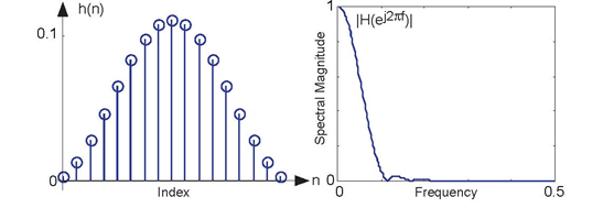
period-17 sinusoid: $h(n)=\frac{1}{17}\left ( 1-\cos\left ( \frac{2\pi n}{17} \right ) \right ),\ n=\left \{ 0,...,16 \right \},$ which makes q = 16. Its frequency response (determined by computing the discrete Fourier transform) is shown in Figure 5.23. To apply, we can select the length of each section so that the frequency-domain filtering approach is maximally efficient: Choose the section length N_xso that N_x+ q is a power of two. To use a length-64 FFT, each section must be 48 samples long. Filtering with the difference equation would require 33 computations per output while the frequency domain requires a little over 16; this frequency-domain implementation is over twice as fast! Figure 5.22 shows how frequency-domain filtering works.

Figure 5.23

The figure shows the unit-sample response of a length-17 Hanning filter on the left and the frequency response on the right. This filter functions as a lowpass filter having a cutoff frequency of about 0.1

We note that the noise has been dramatically reduced, with a sinusoid now clearly visible in the filtered output. Some residual noise remains because noise components within the filter's passband appear in the output as well as the signal.

Exercise 5.15.2

Note that when compared to the input signal's sinusoidal component, the output's sinusoidal component seems to be delayed. What is the source of this delay? Can it be removed?

2118 reads

You are here

Efficiency of Frequency-Domain Filtering