


We know how to acquire analog signals for digital processing (pre-filtering), sampling (The Sampling Theorem), and A/D conversion (Analog-to-Digital Conversion) and to compute spectra of discrete-time signals (using the FFT algorithm (Fast Fourier Transform (FFT)), let's put these various components together to learn how the spectrogram shown in Figure 5.14 (Speech Spectrogram), which is used to analyze speech (Modeling the Speech Signal), is calculated. The speech was sampled at a rate of 11.025 kHz and passed through a 16-bit A/D converter.
POINT OF INTEREST: Music compact discs (CDs) encode their signals at a sampling rate of 44.1 kHz. We'll learn the rationale for this number later. The 11.025 kHz sampling rate for the speech is 1/4 of the CD sampling rate, and was the lowest available sampling rate commensurate with speech signal bandwidths available on my computer.
Exercise 5.10.1
Looking at Figure 5.14 (Speech Spectrogram) the signal lasted a little over 1.2 seconds. How long was the sampled signal (in terms of samples)? What was the datarate during the sampling process in bps (bits per second)? Assuming the computer storage is organized in terms of bytes (8-bit quantities), how many bytes of computer memory does the speech consume?
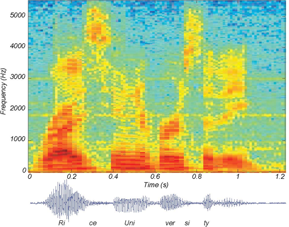
The resulting discrete-time signal, shown in the bottom of Figure 5.14 (Speech Spectrogram), clearly changes its character with time. To display these spectral changes, the long signal was sectioned into frames: comparatively short, contiguous groups of samples. Conceptually, a Fourier transform of each frame is calculated using the FFT. Each frame is not so long that signifcant signal variations are retained within a frame, but not so short that we lose the signal's spectral character. Roughly speaking, the speech signal's spectrum is evaluated over successive time segments and stacked side by side so that the x-axis corresponds to time and the y-axis frequency, with color indicating the spectral amplitude.
An important detail emerges when we examine each framed signal (Figure 5.15 (Spectrogram Hanning vs. Rectangular)).
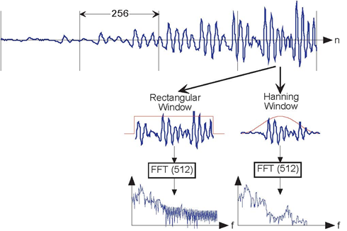
The top waveform is a segment 1024 samples long taken from the beginning of the "Rice University" phrase. Computing Figure 5.14 (Speech Spectrogram) involved creating frames, here demarked by the vertical lines, that were 256 samples long and _nding the spectrum of each. If a rectangular window is applied (corresponding to extracting a frame from the signal), oscillations appear in the spectrum (middle of bottom row). Applying a Hanning window gracefully tapers the signal toward frame edges, thereby yielding a more accurate computation of the signal's spectrum at that moment of time.
At the frame's edges, the signal may change very abruptly, a feature not present in the original signal. A transform of such a segment reveals a curious oscillation in the spectrum, an artifact
directly related to this sharp amplitude change. A better way to frame signals for spectrograms is to apply a window: Shape the signal values within a frame so
that the signal decays gracefully as it nears the edges. This shaping is accomplished by multiplying the framed signal by the sequence w (n). In sectioning the signal, we essentially applied a
rectangular window: w (n)=1, 0 ≤ n
≤ N −1. A much more graceful window
is the Hanning window; it has the cosine shape  As shown in Figure 5.15 (Spectrogram Hanning vs.
Rectangular), this shaping greatly reduces spurious oscillations in each frame's spectrum. Considering the spectrum of the Hanning windowed frame, we find that the oscillations resulting from
applying the rectangular window obscured a formant (the one located at a little more than half the Nyquist frequency).
As shown in Figure 5.15 (Spectrogram Hanning vs.
Rectangular), this shaping greatly reduces spurious oscillations in each frame's spectrum. Considering the spectrum of the Hanning windowed frame, we find that the oscillations resulting from
applying the rectangular window obscured a formant (the one located at a little more than half the Nyquist frequency).
Exercise 5.10.2
What might be the source of these oscillations? To gain some insight, what is the length-2N discrete Fourier transform of a length-N pulse? The pulse emulates the rectangular window, and certainly has edges. Compare your answer with the length-2N transform of a length-N Hanning window.
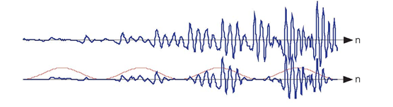
In comparison with the original speech segment shown in the upper plot, the non-overlapped Hanning windowed version shown below it is very ragged. Clearly, spectral information extracted from the bottom plot could well miss important features present in the original.
If you examine the windowed signal sections in sequence to examine windowing's effect on signal amplitude, we see that we have managed to amplitude-modulate the signal with the periodically repeated window (Figure 5.16 (Non-overlapping windows)). To alleviate this problem, frames are overlapped (typically by half a frame duration). This solution requires more Fourier transform calculations than needed by rectangular windowing, but the spectra are much better behaved and spectral changes are much better captured.
The speech signal, such as shown in the speech spectrogram (Figure 5.14: Speech Spectrogram), is sectioned into overlapping, equal-length frames, with a Hanning window applied to each frame. The spectra of each of these is calculated, and displayed in spectrograms with frequency extending vertically, window time location running horizontally, and spectral magnitude color-coded. Figure 5.17 (Overlapping windows for computing spectrograms) illustrates these computations.
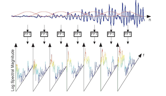
The original speech segment and the sequence of overlapping Hanning windows applied to it are shown in the upper portion. Frames were 256 samples long and a Hanning window was applied with a half-frame overlap. A length-512 FFT of each frame was computed, with the magnitude of the first 257 FFT values displayed vertically, with spectral amplitude values color-coded.
Exercise 5.10.3
Why the specific values of 256 for N and 512 for K? Another issue is how was the length-512 transform of each length-256 windowed frame computed?
- 6128 reads
