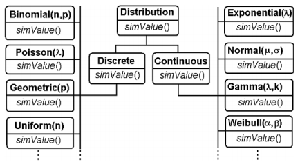
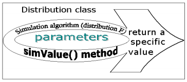
The classical random variables are the simplest stochastic models, also called distributional models, which enter into the composition of other complex models. We propose a hierarchy of Java classes for modelling the classical distributions. Each distribution class encapsulates a particular simValue() method (Figure 3.3).

Each distribution is determined by a set parameters and a distribution function. Based onthese elements we defined a Java class for each distribution, obtaining a generic distributional model (Figure 3.4). This Java class is used to create one or more objects, which are instances with particular values for parameters. Also, a simulation algorithm is defined for each class, which is able to generate a specific value for the corresponding distribution. So, there is a set of simulation algorithms belonging to the whole hierarchy of Java classes, these algorithms being implemented via the polymorphic method called simValue(). The particular implementation of the simulation algorithm for each class is based on one or more of the following techniques: the Inverse Transform Technique, the Acceptance-Rejection Technique and the Composition Technique (Ross, 1990).

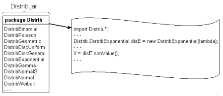
The hierarchy of Java classes for modelling the classical distributions is included in a JAR (JavaARchieve) library. To generate a single value from a particular distribution, it is necessary to import the corresponding distribution class from the library, then to instantiate an object of that class, and finally to call the polymorphic simValue() method based on this object (Figure 3.5). An instance of a particular class can be used to simulate a sequence of values for the corresponding random variable, by calling simValue() as many times as needed.

To make a simulation study for a distribution, it is necessary to generate more values, a sequence of values. One may choose to continually generate additional values, stopping when the efficiency of the simulation is good enough. Generally, one may use the variance of the estimators obtained during the simulation study to decide when to stop the generation of additional values. For example, if the objective is to estimate the mean value μ =E(Xi), i = 0, 1, 2, ..., one may continue to generate new data values until one has generated a number of data values for which the estimate of the standard error is less than an acceptable value.
- 2608 reads


