


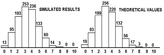
To make a simulation study for a distribution, it is necessary to generate more values, a sequence of values. The learner has the possibility to interactively select a distribution, to set some parameters, to visualize the results of a simulation and to form some conclusions. For example, the learner may choose to generate N = 995 values from previous binomial distribution B (11, 0.3) and to visualize them in a column format. In addition, the learner may visually verify the results of a simulation by comparing them with theoretical values, computed by theoretical formulae (Figure 3.17). There is an obvious relation between theoretical values and the values presented in (Figure 3.16), as in the previous scenario we used the binomial model B (11, 0.3).
The learner may choose to continually generate additional values, stopping when the efficiency of the simulation is good enough. Generally, the learner may use the variance of the estimators obtained during the simulation study to decide when to stop the generation of additional values, i.e., when the efficiency of the simulation study is acceptable. The smaller this variance is, the smaller is the amount of simulation needed to obtain a fixed precision. For example, if the objective is to estimate the mean value μ = E(Xi), i=0, 1, 2, ..., the learner should continue to generate new data until are generated n data values for which the estimate of the standard error, SE = s /

, is less than an acceptable value given previously and named Allowed SE, s being the sample standard deviation. Sample means and sample variances are recursively computed. The final values of these parameters, the confidence interval and other statistics are showed as the result of the simulation study. Figure 3.18 shows a comparison of the results for two simulations from binomial distribution B (11, 0.3), first simulation with allowed standard error of 0.1, and second simulation with allowed standard error of 0.05.
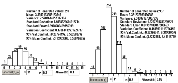
The number of generated values is determined by the value Allowed SE introduced by the learner, as the simulation stops when the condition s / ≤ Allowed SE is true. For the left side simulation, with allowed
standard error of 0.1, are generated 259 values, while for the right side simulation, with allowed standard error of 0.05, are generated 937 values.
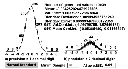
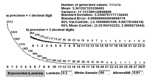
When simulate from a continuous random variable X, a generated value xϵX is approximated with a given precision expressed by the number of decimal digits after the decimal point. The learner has the possibility to choose a precision of one, two, or even more decimal digits. If a coarse approximation is accepted, no decimals are considered and the real value x is approximated by int(x), that is by integer part of the x. In this case the continuous random variable X is rudely approximated by a discrete one, and the results of a simulation can be graphically expressed in a segmented line format, each segment joining the top sides of two neighbouring columns. If a precision of one decimal digit is selected, a more refined segmented line can more precisely visualize the results of the same simulation. With a precision of two decimal digits, a more refined visualization is obtained. The higher this precision is, the higher is the resolution realized in visualization. Figure 3.19,visualized with a precision of one decimal digit, versus a precision of two decimal digits. compares two visualizations for the same set of generated values from the standard normal distribution N(0, 1), the first visualization being with a precision of one decimal digit (Figure 3.19),visualized with a precision of one decimal digit, versus a precision of two decimal digits., graph a), and the second with a precision of two decimal digits (Figure 3.19),visualized with a precision of one decimal digit, versus a precision of two decimal digits., graph b). As can be seen in this figure, when the precision grows with one decimal digit, the resolution grows ten times. With a precision of one decimal digit, ten numbers are considered between two successive integers, while if the precision is of two decimal digits, one hundred numbers are considered between two successive integers. When necessary, intermediate resolutions can be considered. Figure 3.20,visualized with a precision of one decimal digit, versus a precision of two decimal digits. shows a similar comparison for the exponential distribution with parameter λ = 0.3.
- 1930 reads
