


Figure 8.5 illustrates a
possible relationship between the ATC curves for three different scales of operation. is the average total cost curve associated with a small-sized plant.
  is associated with a somewhat larger plant, and so forth. Obviously, the cost curves to the right correspond to larger
production facilities, given that output is measured on the horizontal axis. If there are economies associated with a larger scale of operation, then the average costs associatedwith producing
larger outputs in a larger plant should be lower than the average costs associated with lower outputs in a smaller plant, assuming that the plants are producing the output levels they were
designed to produce. For this reason, the cost curve
is associated with a somewhat larger plant, and so forth. Obviously, the cost curves to the right correspond to larger
production facilities, given that output is measured on the horizontal axis. If there are economies associated with a larger scale of operation, then the average costs associatedwith producing
larger outputs in a larger plant should be lower than the average costs associated with lower outputs in a smaller plant, assuming that the plants are producing the output levels they were
designed to produce. For this reason, the cost curve  has a segment
that is lower than the lowest segment on
has a segment
that is lower than the lowest segment on  . However, in
Figure 8.5 the cost curve
. However, in
Figure 8.5 the cost curve
 has moved upwards. What behaviours are implied here?
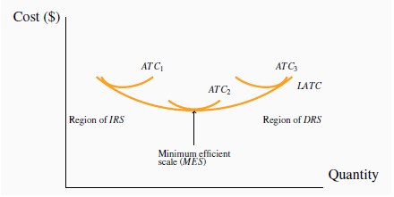
We propose that, beyond some large scale of operation, it becomes increasingly difficult to reap further cost reductions from specialization, organizational economies, or marketing economies.
At such a point, the scale economies are effectively exhausted, and larger plant sizes no longer give rise to lower ATC curves. Figure 8.5 implies that once we get to a production output that plant size 2 is
geared to produce, there are few further scale economies available. And, once we move to producing a very high output (which requires a plant size corresponding to  ), we are actually encountering diseconomies of scale. We stated above that scale
economies reduce unit costs. Correspondingly, diseconomies of scale imply that unit costs increase as a result of the firm’s becoming too large: Perhaps co-ordination difficulties have set in
at the very high output levels, or quality-control monitoring costs have risen.
), we are actually encountering diseconomies of scale. We stated above that scale
economies reduce unit costs. Correspondingly, diseconomies of scale imply that unit costs increase as a result of the firm’s becoming too large: Perhaps co-ordination difficulties have set in
at the very high output levels, or quality-control monitoring costs have risen.
The terms increasing, constant, and decreasing returns to scale underlie the concepts of scale economies and diseconomies: Increasing returns to scale (IRS) implies that, when all inputs are increased by a given proportion, output increases more than proportionately. Constant returns to scale (CRS) implies that output increases in direct proportion to an equal proportionate increase in all inputs. Decreasing returns to scale (DRS) implies that an equal proportionate increase in all inputs leads to a less than proportionate increase in output.
 Increasing returns to scale implies that,
when all inputs are increased by a given proportion, output increases more than proportionately.
Increasing returns to scale implies that,
when all inputs are increased by a given proportion, output increases more than proportionately.
 Constant returns to scale implies that output
increases in direct proportion to an equal proportionate increase in all inputs.
Constant returns to scale implies that output
increases in direct proportion to an equal proportionate increase in all inputs.
 Decreasing returns to scale implies that an
equal proportionate increase in all inputs leads to a less than proportionate increase in output.
Decreasing returns to scale implies that an
equal proportionate increase in all inputs leads to a less than proportionate increase in output.
These are pure production function relationships, but, if the prices of inputs are fixed for producers, they translate directly into the various cost structures illustrated in Figure 8.5. For example, if a doubling of capital and Labour in BDS allows for better production flows than when in the smaller plant, and therefore yields more than double the output, this implies that the cost per snowboard produced must fall in the new plant. In contrast, if a doubling of inputs leads to less than a doubling of outputs then the cost per snowboard must rise. Between these extremes, there is a range of relatively constant unit costs, corresponding to where the production relation is subject to constant returns to scale. In Figure 8.5, the falling unit costs output region has increasing returns to scale, the region that has relatively constant unit costs has constant returns to scale, and the increasing cost region has decreasing returns to scale.
- 2764 reads
