


In Figure 4.5, we examine the
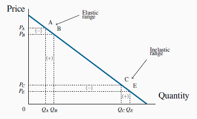
expenditure or revenue impact of a price reduction in two ranges of a linear demand curve. Expenditure, or revenue, is the product of price times quantity. It is, therefore, the area of a
rectangle in a price/quantity diagram. From position A, a price reduction from  to
to  has two impacts. It reduces the revenue that accrues from those
  units already being sold; the negative sign between
  and
and  marks this reduction. But it increases revenue through additional sales from to
  . The area marked with a positive sign between
  and
and  denotes this increase. Will the extra revenue caused by the quantity increase outweigh the loss in revenue associated with each unit sold before the price was reduced? It turns out that at high
prices the positive impact outweighs the negative impact. The intuitive reason is that the existing sales are small and, therefore, we lose a revenue margin on a very limited quantity. The net
impact on total expenditure of the price reduction is positive.
denotes this increase. Will the extra revenue caused by the quantity increase outweigh the loss in revenue associated with each unit sold before the price was reduced? It turns out that at high
prices the positive impact outweighs the negative impact. The intuitive reason is that the existing sales are small and, therefore, we lose a revenue margin on a very limited quantity. The net
impact on total expenditure of the price reduction is positive.
When the price falls from  to
to  , expenditure changes from
  to
to  . In this elastic region expenditure increases, because the loss in revenue on existing units (-) is less than the revenue gain
(+) due to the additional units sold. The opposite occurs in the inelastic region CE.
. In this elastic region expenditure increases, because the loss in revenue on existing units (-) is less than the revenue gain
(+) due to the additional units sold. The opposite occurs in the inelastic region CE.
In contrast, move now to point C and consider a further price reduction from  to
to  .
There is again a dual impact: a loss of revenue on existing sales, and a gain due to additional sales. But in this instance the existing sales
.
There is again a dual impact: a loss of revenue on existing sales, and a gain due to additional sales. But in this instance the existing sales  are large, and therefore the loss of a price margin on these sales is more significant
than the extra revenue that is generated by the additional sales. The net effect is that total expenditure falls.
are large, and therefore the loss of a price margin on these sales is more significant
than the extra revenue that is generated by the additional sales. The net effect is that total expenditure falls.
So if revenue increases in response to price declines at high prices, and falls at low prices, there must be an intermediate region of the demand curve where the composite effects of the price change just offset each other, and no change in revenue results from a price change. It transpires that this occurs at the midpoint of the linear demand curve. Let us confirm this with the help of our example in Table 4.1.
The fourth column of the table contains the point elasticities of demand, and the final column defines the expenditure on the good at the corresponding prices. Point elasticities are very precise; they are measured at a point rather than over a range or an arc. Note next that the point on this linear demand curve where revenue is a maximum corresponds to its midpoint—where the elasticity is unity. This is no coincidence. Price reductions increase revenue so long as demand is elastic, but as soon as demand becomes inelastic such price declines reduce revenues. When does the value become inelastic? Clearly, where the unit elasticity value is crossed. This is illustrated in Figure 4.6, which defines the relationship between total revenue (TR), or total expenditure, and quantity sold in Table 4.1. Total revenue increases initially with quantity, and this increasing quantity of sales comes about as a result of lower prices. At a quantity of 5 units the price is $5.00. This price-quantity combination corresponds to the mid-point of the demand curve.
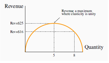
Based upon the data in Table 4.1, revenue increase with quantity sold up to sales of 5 units. Beyond this output, the decline in price that must accompany additional sales causes revenue to decline.
We now have a general conclusion: In order to maximize the possible revenue from the sale of a good or service, it should be priced where the demand elasticity is unity.
Does this conclusion mean that every entrepreneur tries to find this magic region of the demand curve in pricing her product? Not necessarily: Most businesses seek to maximize their profit rather than their revenue, and so they have to focus on cost in addition to sales. We will examine this interaction in later chapters. Secondly, not every firm has control over the price they charge; the price corresponding to the unit elasticity may be too high relative to their competitors’ choices of price. Nonetheless, many firms, especially in the early phase of their life-cycle, focus on revenue growth rather than profit, and so, if they have any power over their price, the choice of the unitelastic price may be appropriate.
Elasticity values are sometimes more informative than diagrams and figures. To see why, consider Figure 4.4 again. Since the demand curve, D, has a “vertical” profile, we tend to think of such a demand as being less elastic than one with a more “horizontal” profile, D'. But that demand curve could be redrawn with the scale of one or both of the axes changed. By using bigger spacing for quantity units (or smaller spacing for the pricing units), a demand curve with a vertical profile could be transformed into one with a horizontal profile! But elasticity calculations do not deceive. The numerical values are always independent of how we mark off units in a diagram. Consequently, when we see a demand curve with a vertical profile, we can indeed say that it is less elastic than a “flatter” demand curve in the same region of the figure. But we cannot form such a conclusion when comparing demand curves for different goods with different units and scales. The beauty of elasticity lies in its honesty!
- 4593 reads
