


Elasticity values are critical in determining the impact of a government’s taxation policies. The spending and taxing activities of the government influence the use of the economy’s resources. By taxing cigarettes, alcohol and fuel, the government can restrict their use; by taxing income, the government influences the amount of time people choose to work. Taxes have a major impact on almost every sector of the Canadian economy.
To illustrate the role played by demand and supply elasticities in tax analysis, we take the example of a sales tax. These can be of the specific or ad valorem type. A specific tax involves a fixed dollar levy per unit of a good sold (e.g., $10 per airport departure). An ad valorem tax is a percentage levy, such as Canada’s Goods and Services tax (e.g., 5 percent on top of the retail price of goods and services). The impact of each type of tax is similar, and we will use the specific tax in our example below.
A layperson’s view of a sales tax is that the tax is borne by the consumer. That is to say, if no sales tax were imposed on the good or service in question, the price paid by the consumer would be the same net of tax price as exists when the tax is in place. Interestingly, this is not always the case. The study of the incidence of taxes is the study of who really bears the tax burden, and this in turn depends upon supply and demand elasticities.
 Tax Incidence describes how the burden of a tax is
shared between buyer and seller.
Tax Incidence describes how the burden of a tax is
shared between buyer and seller.
Consider Figure 4.8 and Figure 4.9, which define an imaginary market for inexpensive wine. Let us suppose that, without a tax, the equilibrium price of a bottle of wine is $5, and Qo is the equilibrium quantity traded. The pre-tax equilibrium is at the point A. The government now imposes a specific tax of $4 per bottle. The impact of the tax is represented by an upward shift in supply of $4: Regardless of the price that the consumer pays, $4 of that price must be remitted to the government. As a consequence, the price paid to the supplier must be $4 less than the consumer price, and this is represented by twin supply curves: one defines the price at which the supplier is willing to supply, and the other is the tax-inclusive supply curve that the consumer faces.
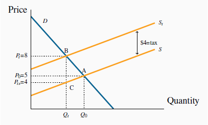
The imposition of a specific tax of $4 shifts the supply curve vertically by $4. The final price at B ( ) increases by $3 over the equilibrium price at A. At the new quantity traded,
  , the supplier gets $4 per unit (
 ), the government gets $4 also and the consumer pays $8. The greater part of the incidence
is upon the buyer, on account of the relatively elastic supply curve: his price increases by $3 of the $4 tax.
), the government gets $4 also and the consumer pays $8. The greater part of the incidence
is upon the buyer, on account of the relatively elastic supply curve: his price increases by $3 of the $4 tax.
The introduction of the tax in Figure 4.8 means that consumers now face the supply curve St . The new equilibrium is at point B. Note that the price has increased by less than the full amount of the tax—in this example it has increased by $3. This is because the reduced quantity at B is provided at a lower supply price: The supplier is willing to supply the quantity Qt at a price defined by C ($4), which is lower than A ($5).
So what is the incidence of the $4 tax? Since the market price has increased from $5 to $8, and the price obtained by the supplier has fallen by $1, we say that the incidence of the tax falls mainly on the consumer: the price to the consumer has risen by three dollars and the price received by the supplier has fallen by just one dollar.
Consider now Figure 4.9, where the supply curve is less elastic, and the demand curve is unchanged. Again the supply curve must shift upward with the imposition of the $4 specific tax. But here the price received by the supplier is lower than in Figure 4.8, and the price paid by the consumer does not rise as much – the incidence is different. The consumer faces a price increase that is one-quarter, rather than three-quarters, of the tax value. The supplier faces a lower supply price, and bears a higher share of the tax.
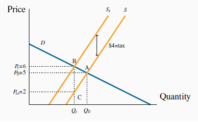
The imposition of a specific tax of $4 shifts the supply curve vertically by $4. The final price at B ( ) increases by $1 over the no-tax price at A. At the new quantity traded,
  , the supplier gets $2 per unit (
 ), the government gets $4 also and the consumer pays $6. The greater part of the incidence
is upon the supplier, on account of the relatively inelastic supply.
), the government gets $4 also and the consumer pays $6. The greater part of the incidence
is upon the supplier, on account of the relatively inelastic supply.
We can draw conclude from this example that, for any given demand, the more elastic is supply, the greater is the price increase in response to a given tax. Furthermore, a more elastic supply curve means that the incidence falls more on the consumer; while a less elastic supply curve means the incidence falls more on the supplier. This conclusion can be verified by drawing a third version of Figure 4.8 and Figure 4.9, in which the supply curve is horizontal – perfectly elastic. When the tax is imposed the price to the consumer increases by the full value of the tax, and the full incidence falls on the buyer. While this case corresponds to the layperson’s intuition of the incidence of a tax, economists recognize it as a special case of the more general outcome, where the incidence falls on both the supply side and the demand side.
These are key results in the theory of taxation. It is equally the case that the incidence of the tax depends upon the demand elasticity. In Figure 4.8 and Figure 4.9 we used the same demand curve. However, it is not difficult to see that, if we were to redo the exercise with a demand curve of a different elasticity, the incidence would not be identical. At the same time, the general result on supply elasticities still holds. We will return to this material in Welfare economics and externalities.
- 5865 reads
