


There are three main ways in which polluters can be controlled. One involves issuing direct controls; the other two involve incentives—in the form of pollution taxes, or on tradable “permits” to pollute.
To see how these different policies operate, consider first Figure 5.7. It is a standard diagram in environmental economics, and is somewhat similar to our supply and demand curves. On the horizontal axis is measured the quantity of environmental damage or pollution, and on the vertical axis its dollar value or cost. The upward-sloping damage curve represents the cost to society of each additional unit of pollution or gas, and it is therefore called a marginal damage curve. It is positively sloped to reflect the reality that, at low levels of emissions, the damage of one more unit is less than at higher levels. In terms of our earlier discussion, this means that an increase in GHGs of 10 ppm when concentrations are at 300 ppm may be less damaging than a corresponding increase when concentrations are at 500 ppm.
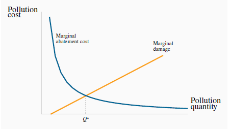
Q* represents the optimal amount of pollution. More than this would involve additional social costs because damages exceed abatement costs. Coversely, less than Q* would require an abatement cost that exceeds the reduction in damage.
 The marginal damage curve reflects the cost to
society of an additional unit of pollution.
The marginal damage curve reflects the cost to
society of an additional unit of pollution.
The second curve is the abatement curve. It reflects the cost of reducing emissions by one unit, and is therefore called a marginal abatement curve. This curve has a negative slope indicating that, as we reduce the total quantity of pollution produced, the cost of further unit reductions rises. This shape corresponds to reality. For example, halving the emissions of pollutants and gases from automobiles may be achieved by adding a catalytic converter and reducing the amount of lead in gasoline. But reducing those emissions all the way to zero requires the development of major new technologies such as electric cars—an enormously more costly undertaking.
 The marginal abatement curve reflects the cost to
society of reducing the quantity of pollution by one unit.
The marginal abatement curve reflects the cost to
society of reducing the quantity of pollution by one unit.
If producers are unconstrained in the amount of pollution they produce, they may produce more than what we will show is the optimal amount – corresponding to Q*. This amount is optimal in the sense that at levels greater than Q* the damage exceeds the cost of reducing the emissions. However, reducing emissions by one unit below Q* would mean incurring a cost per unit reduction that exceeds the benefit of that reduction. Another way of illustrating this is to observe that at a level of pollution above Q* the cost of reducing it is less than the damage it inflicts, and therefore a net gain accrues to society as a result of the reduction. But to reduce pollution below Q* would involve an abatement cost greater than the reduction in pollution damage and therefore no net gain to society. This constitutes a first rule in optimal pollution policy.
An optimal quantity of pollution occurs when the marginal cost of abatement equals the marginal damage.
A second guiding principle emerges by considering a situation in which some firms are relative ‘clean’ and others are ‘dirty’. More specifically, a clean firm A may have already invested in new equipment that uses less energy per unit of output produced, or emits fewer pollutants per unit of output. In contrast the dirty firm B uses older dirtier technology. Suppose furthermore that these two firms form a particular sector of the economy and that the government sets a limit on total pollution from this sector, and that this limit is less than what the two firms are currently producing. What is the least costly method to meet the target?
The intuitive answer to this question goes as follows: in order to reduce pollution at least cost to the sector, calculate what it would cost each firm to reduce pollution from its present level. Then implement a system so that the firm with the least cost of reduction is the first to act. In this case the ‘dirty’ firm will likely have a lower cost of abatement since it has not yet upgraded its physical plant. This leads to a second rule in pollution policy:
With many polluters, the least cost policy to society requires producers with the lowest abatement costs to act first.
This principle implies that policies which impose the same emission limits on firms may not be the least costly manner of achieving a target level of pollution. Let us now consider the use of tradable permits and corrective/carbon taxes as policy instruments. These are market-based systems aimed at reducing GHGs.
 Tradable permits and corrective/carbon
taxes are market-based systems aimed at reducing GHGs.
Tradable permits and corrective/carbon
taxes are market-based systems aimed at reducing GHGs.
- 1634 reads
