


The demand curves developed in The classical marketplace – demand and supply can be related to the foregoing utility analysis. In our example, Neal purchased four lift tickets at Whistler when the price was $30. We can think of this combination as one point on his demand curve, where the “other things kept constant” are the price of jazz, his income, his tastes, etc.
Suppose now that the price of a lift ticket increased to $40. How could we find another point on his demand curve corresponding to this price, using the information in Table 6.1? The marginal utility per dollar associated with each
visit to Whistler could be recomputed by dividing the values in column 4 by 40 rather than 30, yielding a new column 6. We would then determine a new allocation of his budget between the two
goods that would maximize utility. After such a calculation we would find that he makes three visits to Whistler and four jazz-club visits. Thus, the combination ( = $40 ,
  = 3) is another point on his demand curve. Note that this allocation exactly exhausts his $200 budget.
By setting the price equal to $20, this exercise could be performed again, and the outcome will be a quantity demanded of lift tickets equal to seven (plus three jazz club visits). Thus, the
combination ( = $20 ,
  = 7) is another point on his demand curve. Figure 6.5 plots a demand curve going through these
three points.
= 7) is another point on his demand curve. Figure 6.5 plots a demand curve going through these
three points.
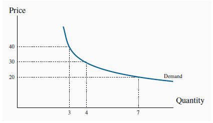
When P = $30, the consumer finds the quantity such that MU/P is equal for all purchases. The corresponding quantity purchased is 4 tickets. At prices of $40 and $20 the equilibrium condition implies quantities of 3 and 7 respectively.
By repeating this exercise for many different prices, the demand curve is established. We have now linked the demand curve to utility theory.
- 1768 reads
